
Introduction
This paper reports our work in the EU-SENSE project. EU-SENSE is sponsored by the European Commission1 and aims to (1) contribute to a better situational awareness of CBRN practitioners, (2) improve the detection capabilities using a novel network of chemical sensors and (3) showcase the usability of the EU-SENSE network.
During the project, a network of chemical point sensors was developed. This network consists of sensor nodes, where each node is equipped with different sensor technologies: IMS,2 EC,3 PID,4 FPD5 and MO6 Sensor array (for a technology overview, see for example Sferopoulos (2009). The idea is to place such a network in an area of interest and
to detect a chemical attack;
to estimate the concentration of the detected substance;
to infer information about the source that released the substance;
to predict the hazard resulting from that source.
Examples for these kinds of scenarios could be mass events such as sport events, open-air festivals, etc. The aim in such a scenario is to detect a CBRN attack as early and reliable as possible. This detection should be sensitive but also reliable. This requirement is usually difficult to achieve since there is a trade-off between sensitivity and reliability of a sensor. The more sensitive a sensor is the higher is its probability of producing false positives. With a network of sensors however, the expectation is to reduce the number false alarms.
The focus of this paper is on the data fusion aspects, the statistical and machine learning approaches that were used in the project. We have been focussing in particular on the first two tasks mentioned, that is detection and concentration estimation. Source term estimation and hazard prediction was at ask in another part of the project, led by 7Swedish Defence Research Agency, Member of the EU-SENSE Consortium.FOI.7
The goal of reliable detection was achieved by a two-step procedure: First, a sensitive anomaly or change detection was applied. Then, an identification step followed, making the detection reliable and quantifiable. The anomaly detection uses straightforward statistical methods. Bayesian inference proved to be a robust tool for data fusion and classification as well as regression.
Network and Hardware
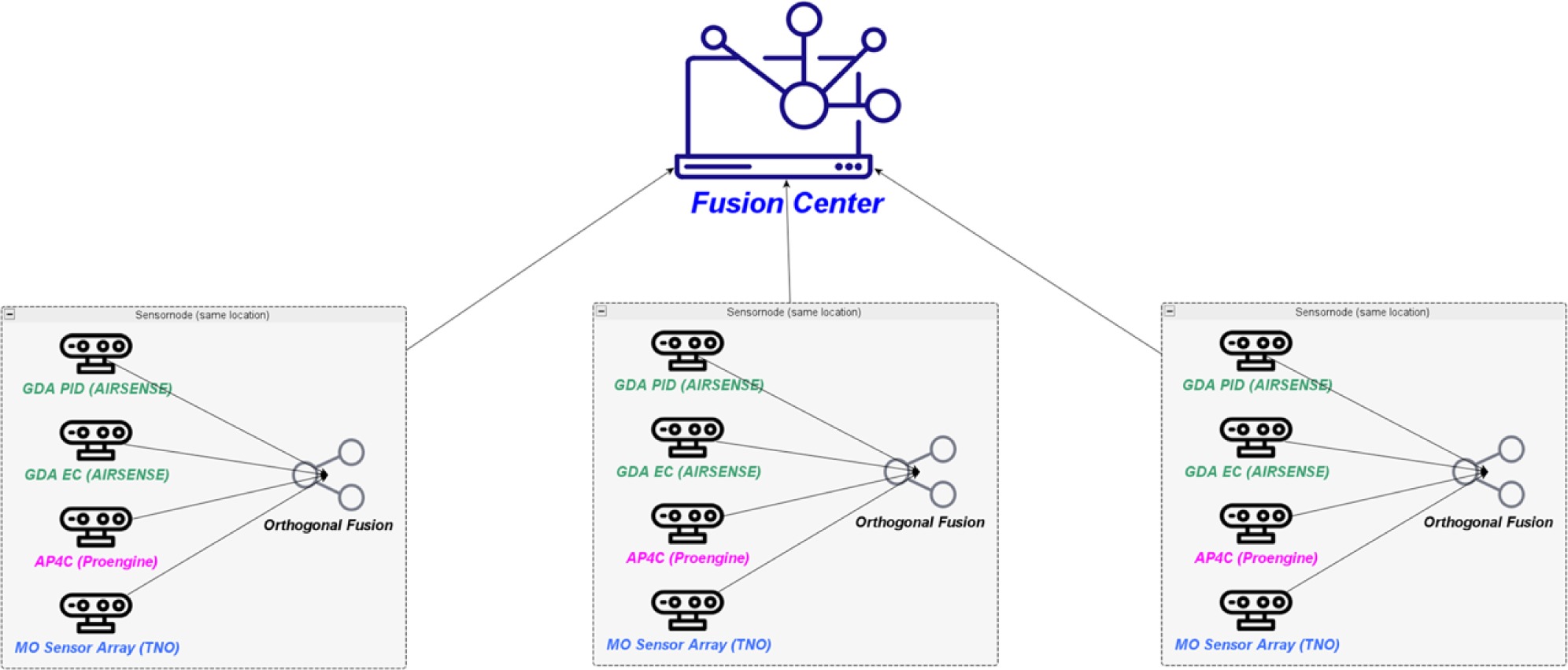
The prototypal network developed in EU-SENSE consists of three sensor nodes (Fig. 1). Three nodes are somewhat sparse for monitoring a “high visibility mass event” but the focus was on building a network with real CBRN Detectors in order to see which improvement sensor data fusion can achieve. Due to budgetary restrictions, it was not possible to use a larger set of sensors.
Each node was equipped with the following sensors, as shown in Table 1.
Table 1.
List of sensors within a single node.
| GDA-P(IMS (H2O) + EC) | Producer: AIRSENSE Analyticsa |
| GDA-P(IMS (NH3) + PID) | Producer: AIRSENSE Analytics |
| AP4C(FPD) | Producer: Proengin |
| MO Sensor Array | Prototype: TNO |
The GDA-P and AP4C are mature chemical detectors. The MO Sensor array is an experimental system still under development. The AP4C provides five response channels corresponding to specific substance classes (As, CH, HNO, P, S). The two GDA-P instruments combine an IMS with one other sensor (PID or EC) respectively: The IMS does not provide merely a simple sensor response but a spectrum (drift-times/mobilities) that allows for identification. In combination with a second detector (EC, PID), they form an orthogonal detector themselves. Figure 2 shows one of the three nodes.
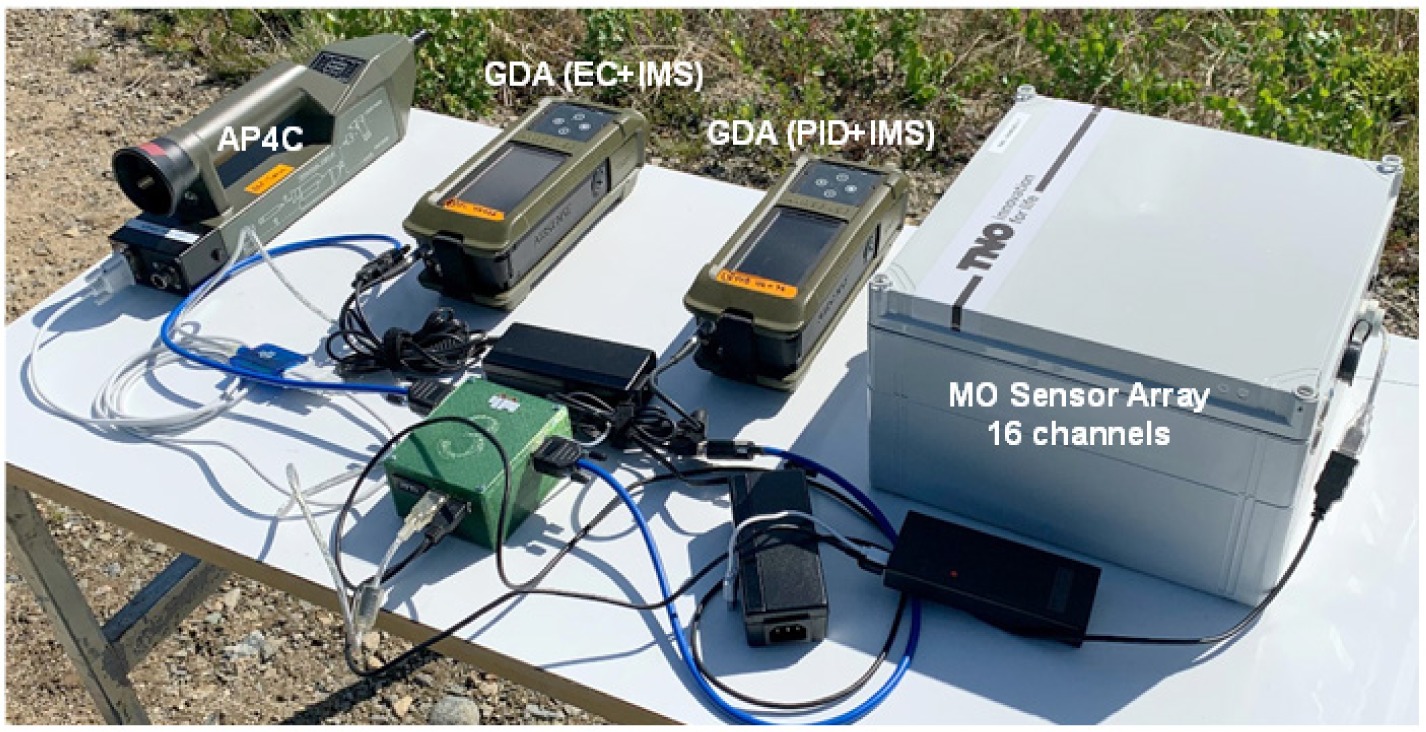
The green box is the node controller. Its task is to receive the sensors responses and forward them to the network of sensors controller.
The following diagram shows the overall system architecture (Figure 3).
Figure 3.
Network architecture (ITTI a).
aITTI Sp. z o.o. – Consortium Lead and responsible for technical architecture.

The diagram also shows other modules of EU-SENSE. However, the focus of this paper is on data fusion. Other aspects of the EU-SENSE network are covered in specific project reports.
Experiments and Data Model
In order to perform data fusion and for machine learning algorithms, relevant data is required. Within the EU-SENSE project, a number of experiments were conducted in the laboratory and outdoors as well.
The measurement campaigns started at the end of 2019 (Norway FFI). However, the process of setting up complex sensing equipment and experiments was error-prone and time-consuming. It was not until mid-December when the first useful measurement results were available. Table 2 shows the time schedule of the measurements.
Table 2.
Schedule of measurements.
Laboratory measurements were planned and started in Spring 2020. During Summer 2020, FOI and SGSP1 conducted outdoor measurements. In November and December, TNO2 conducted measurements, outdoor and in a laboratory as well. It was also extremely helpful that they were able to perform measurements in a breeze tunnel.
Recently, in May 2021, FFI3 again conducted outdoor measurements in Norway. The results served as test data.
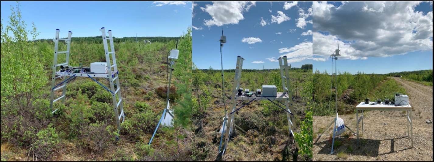
Figures 4 and 5 give an impression of the FOI measurement setup.


The measurements at a sampling rate of approx. 1 Hz produce a lot of data.
The essential part of the responses (w/o the many support values like flags, temperatures, pressures, etc.) are:
These form a time series of approx. 2000 values which are continuously processed by the data-fusion functions of the system.
Task: Sensor Data Fusion
According to (Mitchell, 2007, p. 3), multi-sensor data fusion is defined as follows: The theory, techniques and tools which are used for combining sensor data or data derived from sensory data, into a common representational format. In performing sensor fusion our aim is to improve the quality of the information, so that it is, in some sense, better than would be possible if the data sources were used individually.
This is a very general definition and to make it more specific, it has to be explained what kind of information is needed in the EU-SENSE context. The information EU-SENSE is interested in:
detection of an incident, that is the release of a harmful substance concentration;
estimation of the concentration of the released agent;
estimation of the source (location, strength) of the released agent;
hazard prediction.
Therefore, the above definition of multi-sensor data fusion translated into the EU-SENSE context aims at improving the quality of the detection, concentration/source-term estimation and prediction of the area under threat, so that it is, in some sense, better than would be possible if the data sources were used individually.
Detection (in the sense of “detect-to-warn”) is the decision regarding whether an (real) incident has occurred or not within a timeframe that still allows preventive action to be taken. Incident means the presence of a harmful substance concentration. In this case, the detection should follow as early and reliably as possible. Long delays (e.g. minutes) are usually not acceptable.
In addition, the concentration estimation should also be better solved using sensor data fusion.
In order to make the detection sensitive and simultaneously reliable, we perform detection in several steps, namely:
Anomaly Detection – detecting if the signal is changing;
Classification – pre-classification into substance groups;
Identification – determining the substance.
The first step ‘anomaly detection’ ensures that detection is sensitive. However, it has to be verified that this anomaly is a real event. The next steps accomplish this verification: identification/classification. All these steps provide results in a few seconds.
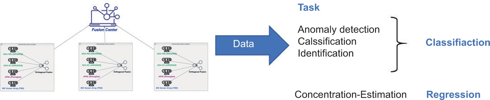
Mathematically, our data fusion solves classification and regression tasks. It is classification when you want to decide whether a certain sensor response is a significant change, an anomaly. Obviously, it is also classification when you decide which agent or which agent class is released. However, concentration estimation is a regression task. A certain number of µg/m3 or ppm need to be known.
Detection
As mentioned, detection is performed first by an anomaly detection, that is detection of a change, an unusual, possibly harmful situation, in the incoming time series of sensor responses. The method we have chosen is sensitive but not specific. This makes it necessary to verify whether the detected anomaly is really a harmful incident or is merely a false positive. The following chapters describe this detection process in more detail.
Anomaly Detection
Anomaly Detection has been and still is a large area of research and development. In the domains of banking, fraud and intrusion detection, cyber security, predictive maintenance and others, many different problems have been researched. Characteristics of anomaly detection problems are manifold and so are the approaches to solve these problems (see e.g. Mehrotra, Mohan, and Huang, 2017).
The following two sections give a short description of how anomaly detection is implemented in the EU-SENSE project and show its performance based on experimental data.
Method
Anomaly detection is based on raw sensor data collected from the individual sensors. These sensors are combined into “sensor nodes” and, at a higher level, a network of sensor nodes. Therefore, the anomaly detection can take place on sensor level, at node level and/or at the network level. We decided to use a straightforward statistical, distance-based approach which compares incoming response values against (multi-variate) probability distributions learned continuously from previously seen data (online learning) in different schemes.
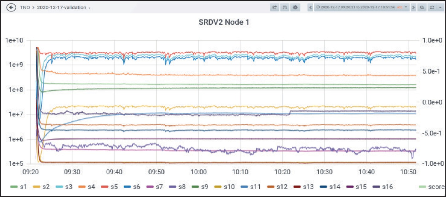
The results of anomaly detection are, eventually, new (one-dimensional) time series (on sensor level, node level etc.) of anomaly scores. These anomaly scores are sensitive. This is due to the multivariate nature of the many response channels in some sensors or in the whole node. If a signal is caused by an incident (or whatever), then it is common that multiple sensor channels will respond to this signal. This can reinforce the distance measure, that is the anomaly score. Figure 8 shows an early example. The upper graph shows the responses of the 16 MO Sensor channels and the lower graph shows (among others) the time series with the anomaly score in red.
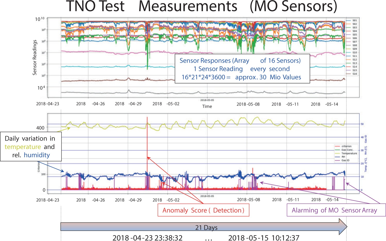
In particular, when some signal appears in multiple channels (upper graph), then this corresponds to a very significant peak in the red anomaly score (lower graph).
Since there are three nodes with quite a lot of sensors involved, the number of different scores gets quite complex. Table 3 shows the designations of the single-sensor scores, used in the following graphs and explanations:
Table 3.
Score designation.
| NODE | ||||
|---|---|---|---|---|
| 1 | 2 | 3 | ||
| IMS H2O | + | Score_1 | Score_1 | Score_1 |
| - | Score_2 | Score_2 | Score_2 | |
| IMS NH3 | + | Score_1 | Score_1 | Score_1 |
| - | Score_2 | Score_2 | Score_2 | |
| EC | Score | Score | Score | |
| PID | Score | Score | Score | |
| FPD | Score | Score | Score | |
| MO Array | Score | Score | Score | |
To keep the designation simple, only the IMS scores have an index to distinguish between the positive (Score_1) and the negative spectrum (Score_2). Further, there are sensor-vs-sensor scores, that is the scores that are computed for pairs of sensors in the network. Since we do not use those in the following figures, we omit the details here. All this makes the tracing of an anomaly a bit confusing.
Experimental Review of the anomaly detector
This section shows the performance of the previously described anomaly detection. It is based on experimental data sets that were obtained during the measurement campaigns of EU-SENSE. The aim is to show that the anomaly detection robustly detects a real incident and that the anomaly detection is sensitive. However, the latter implies that False Positives are unavoidable:
In this context, it is interesting to reflect for a moment what a false alarm actually is. Is it a false alarm when there is a harmless concentration of a substance in the air, for instance phosphorus containing fertilizers and the FPD (P channel) responds to that? The FPD obviously does exactly what it is supposed to do and, from this perspective, this not a false alarm. However, it is a false alarm for emergency personnel since the substance is harmless. Therefore, it is necessary to verify, whether an anomaly is a real incident. The following discussion contains examples for the above-mentioned anomaly cases.
Anomaly detection caused by a real incident
The first example is from the TNO experiment on 17 December 2020, which was recorded as a dedicated validation data set. The experiment took place in a breeze tunnel environment, where it is possible to generate defined concentrations, while at the same time exposing the EU-SENSE sensor nodes to the same environment. In this experiment, Node 1 was placed outside the tunnel, that is, it was not exposed to the test substances. Node 2 (with FPD) and Node 3 (without FPD) were inside the tunnel, that is to say exposed to the same environment and substance releases. The experiment consisted of
a start-phase without a release.
followed by a NH3 release with a rather low concentration (below AEGL-11).
a TEP release on top of the continuing NH3 flow with fluctuating concentrations (two peaks; assumed harmful).
a final phase where first the TEP release and later the NH3 release were shut down.
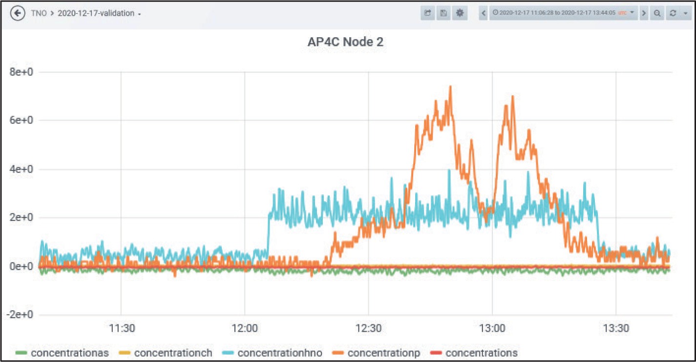
Figure 9 shows the original, recorded response channels of the FPD on Node 2. These responses reflect the concentration development over time. The HNO channel (cyan) qualitatively represents the NH3 concentration; the P channel (orange) qualitatively represents the TEP concentration.
For a test of the Anomaly Detection part, a (real-time) replay was performed on 11.05.2021 with the original data from this experiment using all three nodes. Replay means that the original time series is read and replayed with modified time and processed with the usual data fusion functions. Figure 10 shows this for the FPD.
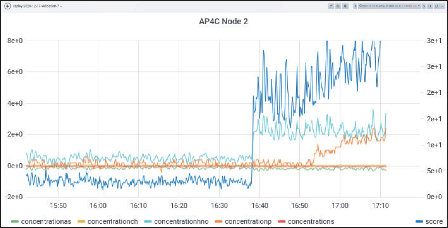
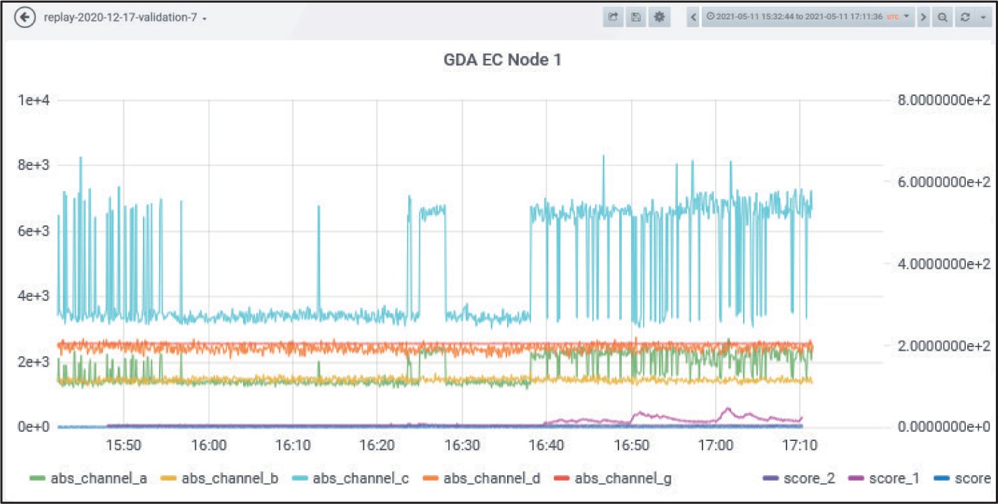
It can be clearly seen that the blue anomaly score rockets upward when the NH3 signal starts. Also, note that the score increases further when the orange response (due to TEP signal) increases. The appearance of the NH3 signal is also detected by other sensors, for example by the IMS (H2O) shown in Figure 11.

In this case, there are three scores: score (EC), score_1, score_2 (pos./neg. spectrum). Here, only score_1 rockets upward. According to our naming conventions, score_1 arises from the positive spectrum of the IMS. The two other scores do not contribute at all. They correspond to the negative IMS spectrum (purple) and to the electro chemical cell (blue).
Does the IMS (NH3) detect the NH3 signal? No, because this is NH3 doped and hence not able to detect NH3. Here are the responses and scores of the IMS NH3 + PID.
In the picture of the IMS NH3 + PID responses (Figure 12), there is no increase of the anomaly scores at 16:38 when the NH3 is released. However, there is a significant increase of score_1 (IMS pos. spectrum) starting at approximately 16:59. At that time, the gradually increasing TEP release started. The increase in score is significant but much smaller than for the IMS H2O at the NH3 release. The different scale of the right y-axis should be noted (the absolute score values can be compared). The PID score ‘score’ shows no anomaly since the NH3, as well as the TEP concentration, are below the detection limit of the PID.

The examples presented so far show that the anomaly detector is able to discover real incidents even with rather low concentrations involved. Sometimes, this is not desirable, namely when the concentrations are so low that they are not relevant.
Anomaly caused by small concentrations
An example taken again from the breeze tunnel experiment. As mentioned, Node 1 was placed outside the tunnel and should therefore not be exposed to the substances (NH3, TEP). Nevertheless, there was also an anomaly warning on Node 1.
This anomaly was only detected by the IMS (H20). Interestingly, score_1 (IMS positive spectrum) started to increase at approximately 16:39:30, that is to say approximately at the same time NH3 was released. The anomaly score ‘score_1’ was significant but much lower than the corresponding score at Node 2. Therefore, it was suspected that some of the NH3 somehow has reached Node 1 located outside the tunnel (perhaps during preparation activities outside the tunnel). To verify that, we looked at the (positive) spectrum of the IMS H2O. Figure 14 shows this spectrum shortly before and shortly after the detected change.
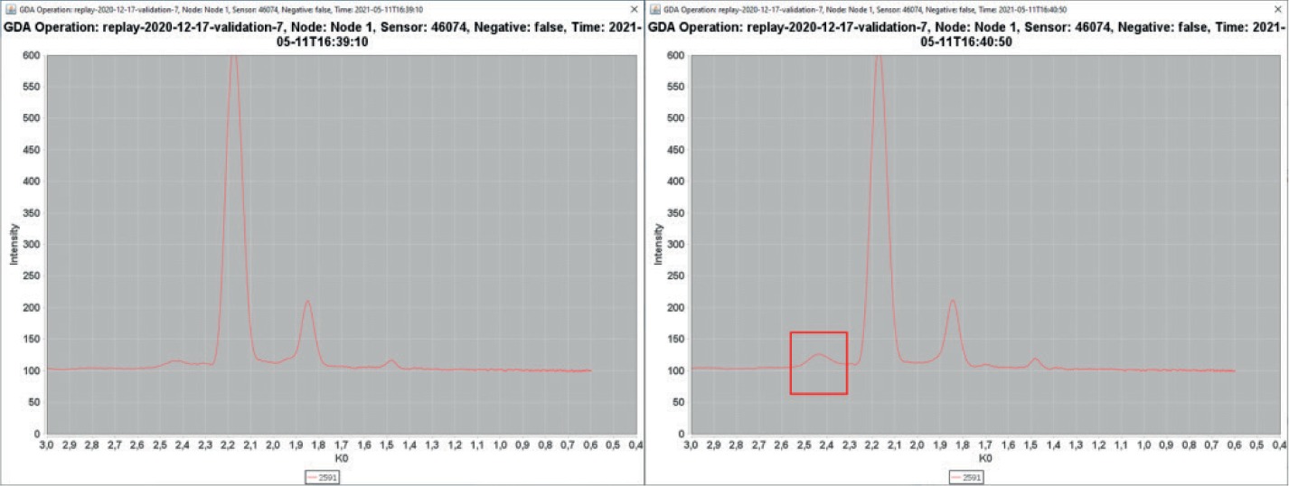
Indeed, at the position where one expects NH3, a small peak is evolving. It seems plausible that a fraction of the NH3 inadvertently escaped the breeze tunnel and caused a response at Node 1.
Anomaly caused by harmless substances
This small, unintended signal detected on Node 1 is also a good example of a harmless signal. Actually, the NH3 concentrations in the tunnel during this experiment were harmless since they were below AEGL-1. The TEP signal that followed later was the actually targeted and assumed harmful release. Other examples of common harmless signals were seen in experimental data from the tests performed in April/May 2021 by FFI. These took place in a half-closed tunnel environment with many short, traffic-induced signals.
Anomaly caused by an artefact
The following example (Figure 15) illustrates where an artefact causes an anomaly warning at sensor level. This occurred during the validation experiment on 2020/12/17. The sensor, which causes the anomaly, was the MO sensor array at Node 1.
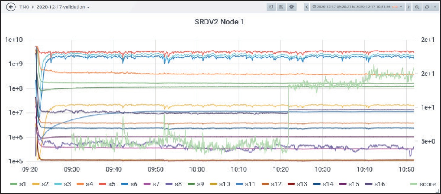
The anomaly does not leap to the eye when looking at the time series of the 16 MO channels. After an adjustment phase (approx. up to 09:35), the development of the time series seems to be a bit noisy but altogether quite inconspicuous. There are peaks and spikes, but the anomaly detector recognised (‘learned’) this as the normal status. However, if you look at the corresponding anomaly score (green) of this sensor, a sharp leap at approximately 10:22 can be seen.
The reason for this leap is a discontinuity in channel 16 of the MO sensor array at 10:22. The channel-16 time series is almost constant with very low noise and no real signal at all. At 10:22 there is a small leap and the series continues again almost constant with extremely low noise. This is a clear change and is correctly recognised by the anomaly detector.
However, the reason for the change is unknown. In addition, the baselines of the 16 channels are slightly changing from experiment to experiment and also differ among sensor instances.
In this example, the baseline of channel 16 changed significantly within the experiment and, therefore, the anomaly detector gave a warning. The anomaly was not due to a real incident. None of the other channels of the MO sensor or any other sensor at Node 1, as well as the other sensors in the network (breeze tunnel; basically controlled environment), showed any conspicuity. Additionally, sudden response level changes on exactly that channel of that specific sensor (and no other sensor at the same time) were encountered during other experiments. We therefore assume this is an example of an anomaly caused by a sensor artefact. There are several more examples of such kinds of anomalies but, for reasons of space, they cannot be discussed here.
To sum up, the anomaly detector is sensitive. It can be applied at sensor level and also at node level and network level. However, according to our experience, it is sufficient to consider only the sensor level. The node level and network level do not bring much additional benefit to our experience. The anomaly detector is able to detect real incidents but it also detects small signals and artefacts. Therefore, the next step in the detection process is to verify whether an anomaly is a real incident, that is to say classification/identification.
Classification/Identification
The second step in detection of a real incident is identification. Only when a signal is identified as harmful (substance, concentration) can one speak of a real incident and raise an alarm.
Identification is performed for each node because it can be assumed that all sensors at a specific node are exposed to the same agent concentration. This is not necessarily the case for two distant nodes. Identification should make use of all the technologies available at that node, that is to say
In the following we describe two approaches for how we fuse the data from the different sensors in order to perform identification. We call these two approaches “fusion approach” and “stepwise-approach”. Both approaches have to be considered prototypical since the number of substances measured in trials and experiments was limited and only some target substances (namely NH3, TEP, MeS) could be used. Compared to real chemical agents such as sarin, mustard etc. these substances are relatively harmless. It was not possible to build up a practically relevant substance library with many target substances in the project from scratch.
Fusion approach
This approach is the prototypical development through fusion of all available sensor information at a node with Bayesian networks only. The necessary prior knowledge was gained from the experiments in the EU-SENSE project itself (i.e. no knowledge is incorporated from the sensor manufacturer) and therefore limited to two substances, NH3 (TIC example) and TEP (CWA simulant, with assumed high toxicity).
Stepwise approach
This approach relies solely on the existing sensor technology available at the inferring node implicitly including the necessary knowledge of the manufacturer (in the form of substance libraries, not available to the project). It consists of the two steps:
Classification, that is assigning the observation to a substance group (e.g. phosphorus containing agents), thereby narrowing down the whole range of possible substances.
Simultaneous Identification & Concentration Estimation through IMS technology based on existing substance libraries.
Fusion Approach
This approach makes use of Bayesian Networks which process knowledge contained in the so-called conditional probability distributions and prior distributions. This knowledge was derived from training data collected during the TNO experiments in November and December 2020. This paper is not the place to explain these methods in depth. Instead, we refer to the relevant literature to Bayesian Inference available in abundance, see for example Jensen and Nielsen (2007), Mitchell (2007) and Ó Ruanaidh and Fitzgerald (1996).
Bayesian approaches are standard in Multi-Sensor Data-Fusion. Many of the papers on CBRN sensor data fusion deal with Bayesian methods. Many of them are concerned with source term determination, for example Robins and Paul (2005a, p. 8) and Robins, Rapley and Thomas (2005b, p. 7).
Here are just some important terms and concepts of Bayesian networks:
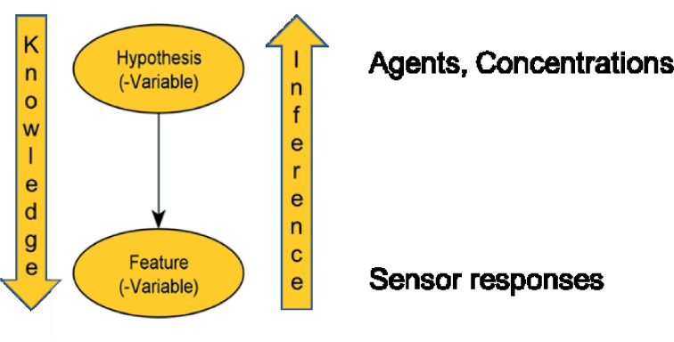
Bayesian inference is about knowledge. The nodes of the network are random Variables (X1, X2, ..., Xn). There are observation variables (also called feature variables) and hypothesis variables. Hypotheses variables in the EU-SENSE context are variables representing the different substances and/or representing the corresponding concentrations. Observation (feature) variables are variables representing the sensor responses.
The knowledge is contained in (conditional) probability distributions of the response variables given a certain substance together with its concentration. This knowledge is used when inferring the substance and concentration from a given observation of the sensor response(s). Simply spoken, the knowledge is “directed” from the hypotheses variables to the observation variables and the inference is “directed” from the observation variables to the hypotheses variables. This is sketched in the following simple “Bayesian network” (Figure 17).
Bayesian network for identification
The core of the identification is the Bayesian Network shown in Figure 18. The hypotheses variables are substance and concentration. Both are discrete variables, that is to say they have a finite number of levels.

The hypothesis variable concentration has four levels, that is to say the concentration values are assigned to four classes corresponding to the AEGL (10 min.) values:
For the hypothesis variable substance, the following substance classes are used:
NH3
TEP
Other: other substance or somehow inconsistent with respect to the implicit knowledge.
None: Not actually a substance; corresponds to a very low signal.
The other nodes of the Bayesian network are observation variables and correspond to sensor response values. Note that not all available sensor response variables are represented in the network. The relevant response values have been identified through a relevance analysis during training time. Of course, this selection is substance specific, that is to say sensor values that neither respond to NH3 nor TEP do not appear here. We used the WEKA tool suite (Waikato Environment for Knowledge Analysis) for the relevance analysis. Despite this down-selection for simplicity reasons, all sensor channels can easily be added here.
The mechanics of this Bayesian network are that the observation variables, the sensor responses, will produce response values after the system has identified an anomaly. Then, with Bayes ‘theorem, the probabilities for the presence of a certain substance and its concentration are calculated. This is called Bayesian inference. In our case: after observing the sensor responses the probabilities for the four substance classes NH3, TEP, Other, None are determined. The knowledge, which enables this inference, is contained in the conditional probabilities such as: given the substance is TEP in a concentration of class MEDIUM, then the sensor responses of the IMS (H2O), positive/negative spectrum, IMS (NH3), positive/negative spectrum, EC, PID, MO sensor array possess certain probability distributions. These (conditional) distributions were determined in the experiments.
Remarks and limitations
The scope of the classification or identification is limited to four substance classes. Unfortunately, no other reliable substance information was available to us in the project. Though the Bayesian network can easily be extended with other substances, we consider this as a proof-of-concept implementation. It should also be noted that despite the fact that the algorithms were implemented in software, they have not been optimised for real-world use. Many aspects to filter out real-world artefacts would have to be considered for this (e.g. baseline correction, smoothing over time). This includes measurement situations (signal side) and sensor artefacts, which perhaps do not occur often. All this requires many more measurements with the sensors in many different environments.
Those real-world artefacts include the behaviour of different instances of the same sensor that maybe too different to model uniquely. This is the reason why there are three different PID sensors as response variables in the Bayesian network in Figure 18. Actually, the Network relates to one node and every node has only one PID. However, the differences in response characteristics of the three PID are too large and they need to be treated as different sensors. When applying the network to a particular node, only the response of the PID for that node needs to be specified. The 5-digit number identifies the proper PID for the node. The other two are not specified. Also generally, the input to the response variables can be partial, that is to say it is not necessary to specify all the response values. The Bayesian inference will nevertheless work properly.
The formulation of the identification problem with the Bayesian network in Figure 18 implies the assumption that the node is exposed to a concentration of a single substance. This will lead to problems when the presented concentration is a mixture of two or more agents. Although the classifier is able to identify NH3 or TEP correctly, it will come out with the classification OTHER when the node is exposed to a mixture of NH3 and TEP. Actually, this is correct since it is not NH3 and it is not TEP. It is a mixture. Nevertheless, this is somehow unsatisfactory from the application point of view. This phenomenon can be observed with the validation dataset recorded by TNO on 17.12.2020. We come back to this during the discussion of the experimental results.
Stepwise approach
The “stepwise-approach” is an engineering approach relying solely on the existing sensor technology at the inferring node including the prior knowledge integrated by the manufacturers. The basic idea is to utilise orthogonal sensor fusion in order to reduce the size of the IMS identification libraries. Narrowing down the set of possible substance candidates avoids false positives (substance identified due to a harmless disturbance signal) as well as confusion of substance candidates (overlaps of drift time windows). The substance libraries contain prior knowledge of the IMS manufacturer. Therefore, no additional experiments/tests are necessary to gather response relationship information etc.
As a first step after an anomaly detection, the classification step derives information about the substance groups.
The following substance groups are used in EU-SENSE (Table 4):
Table 4.
EU-SENSE substance groups.
This information then is used to reduce the substance library and to obtain the IMS results containing simultaneously identification and concentration estimates directly.
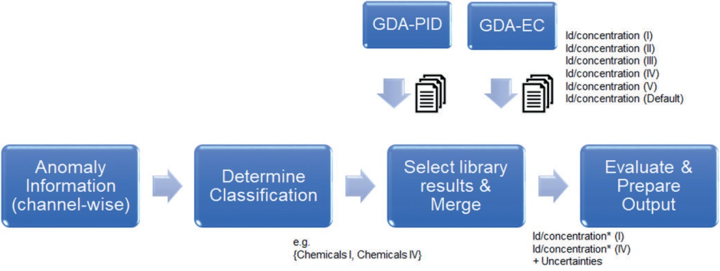
Figure 19 sketches the “stepwise approach”. Because of the Classification to classes I and IV, a sub selection of the identification occurs (it also results from Default, which is always included). The * indicates that the concentration estimates might be fused from the results of both IMS sensors.
Concentration Estimation
The estimation of the concentration of a substance is important for the source term determination as well as for operational reasons. However, concentration estimation is difficult because the underlying physical process (turbulent Diffusion) is chaotic and, hence, fluctuating. Further noise/clutter superimposes the sensor signal resulting in additional uncertainties apart from the uncertainties related to the sensor itself. All this makes concentration determinations rough estimates. Together with the fusion approach comes a coarse classification of the concentration with four discrete levels low, medium, high, very high. This is coarse and, for several reasons, one would like to have a quantitative estimate. Therefore, a separate method was developed to determine the concentration.
Estimating a quantitative concentration from given sensor values is a typical regression problem. Since the concentration determination should use all sensors responses available at a specific node, it is also a fusion problem. This regression/fusion problem again can be solved by a Bayesian network. In contrast to the Bayesian network we discussed before, all variables are now continuous, in particular the hypothesis variable concentration. Figure 20 shows the network for the concentration estimation.
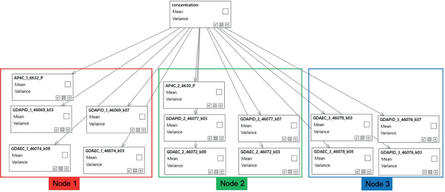
The estimation can start after the identification has happened. Since identification is already accomplished, there is only one hypothesis variable, namely concentration. The parameters are of course substance dependent and the inference result, after putting in all the sensor responses, is the probability distribution of the concentration, characterised by a mean and a variance.
In order to provide this network with knowledge, we need data. Knowledge means how the different sensors respond to the exposure of certain substance concentrations, that is to say quantitative intensity and time characteristics (sensor/substance dependent). Again, the quantitative TNO measurements in the lab (NH3) and breeze tunnel (TEP) in November/December 2020 delivered the necessary data. For both substances, the sensor nodes were completely setup and exposed simultaneously to defined concentrations. There were reference calculations and additional, independent measurements for the concentrations. Several concentration levels were covered in both an upward stair fashion and a downward stair fashion with cleaning phases in between. Based upon this data, we were able to derive the necessary conditional probability distributions and regression parameters containing the knowledge.
For pre-training of the algorithms, a data extraction tool was developed that converted reference data into dedicated training data sets. These datasets were then finally used for training of the Network parameters (mean, standard deviation, regression parameter) for a single sensor, that is the prior knowledge was integrated independently for each sensor. The training algorithm used was an Expectation Maximization (EM) algorithm. This process also demonstrates the extensibility of the approach. Sensors can be integrated step-by-step on top of an existing configuration.
Experimental Review
In the next sections, we discuss some experimental results that show how the classification/identification and concentration algorithms perform in the field.
TNO reference measurements 23.11.2020
As a first test, we execute the concentration estimation and identification on ammonia data recorded by TNO on 23.11.2020. All nodes/sensors were exposed to the same concentrations at the same time. The concentrations were unknown (to us) and the tests were performed in a controlled environment with clean sensors.
Figure 21, showing the raw sensor responses of the FPD (Node 1), gives an impression of the concentration development over time.
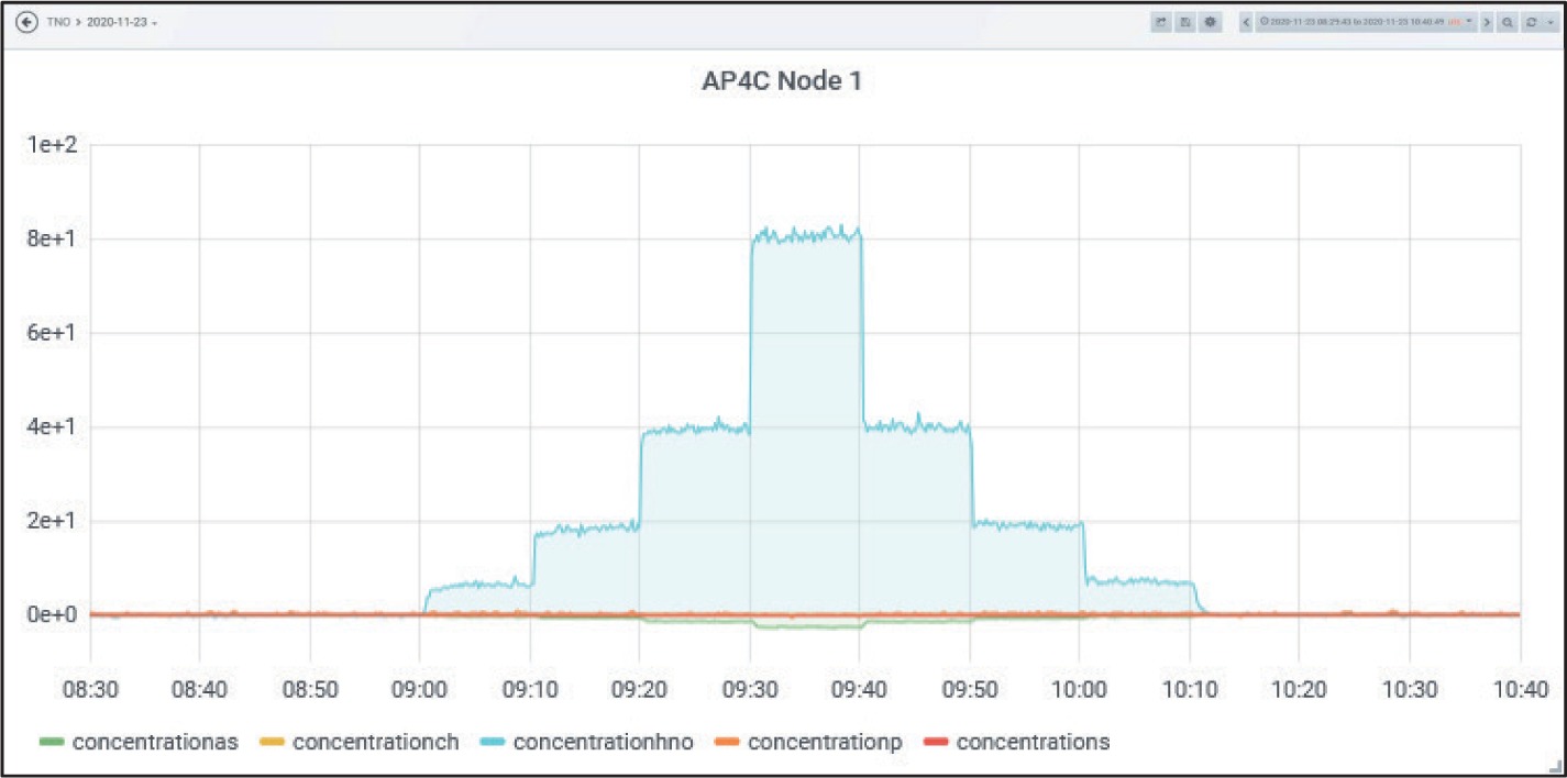
Node 1 was equipped with all available sensors. Node 3 did not contain an FPD. Therefore, on Node 1, information from FPD (HNO), PID and IMS (H2O) was used, while on Node 3 only PID and IMS (H2O) were used for the estimation process (MO-array and EC not integrated here).
Figure 22 shows the corresponding concentration estimates. The right plot is from Node 3, that is without an FPD.

There are slight differences but the results are comparable. At Node 3, the noise is higher. Obviously, the fusion led to the stabilising effect in case more sensors are involved.
To further visualise the effects of orthogonal fusion, Figure 23 (left) shows the result for Node 1 using only data from the IMS (H2O). It seems as if the algorithm based solely on responses from the IMS (H2O) alone overestimates the concentration. In addition, the noise is higher here.
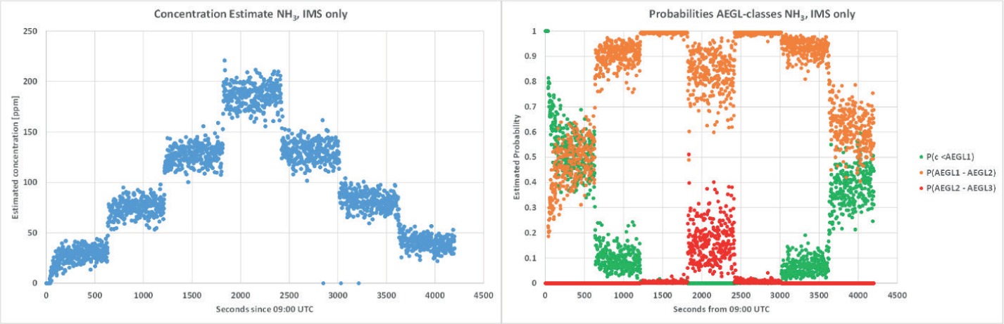
The right graph of Figure 23 shows the estimated probabilities of defined concentration classes. These are derived from the concentration estimation process. The algorithm estimates a probability distribution for the concentration, characterised by a mean and a variance. With this distribution, the probabilities of the concentration classes are calculated (assuming normal distribution).
Blue corresponds to the probability of the concentration in class LOW, that is smaller than AEGL-1 1AEGL (10 min) for NH3: 30 ppm (AEGL-1), 220 ppm (AEGL-2), 2700 ppm (AEGL-3) according to https://www.epa.gov/aegl/ammonia-results-aegl-program (12.11.2021)..1 Orange corresponds to class MEDIUM, that is AEGL-1 < concentration < AEGL-2 and Grey corresponds to class HIGH, that is AEGL-2 < concentration < AEGL-3. This visualises the uncertainty estimate. The corresponding plots for Node 1 (all sensors) and Node 3 (w/o FPD) can be found in Figure 24.
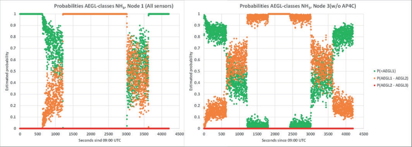
The class probabilities are just a coarsening of the concentration results in Figure 23 (left). The information is essentially the same. In the middle of the up- and down-staircase of concentration, the concentration estimate is MEDIUM, that is between AEGL-1 and AEGL-2 (Figure 24).
These results are all generated from the concentration estimation step.
The identification results in this case are rather unambiguous: For the complete relevant period, they deliver probability 1 or almost 1 for NH3. See Figure 25.
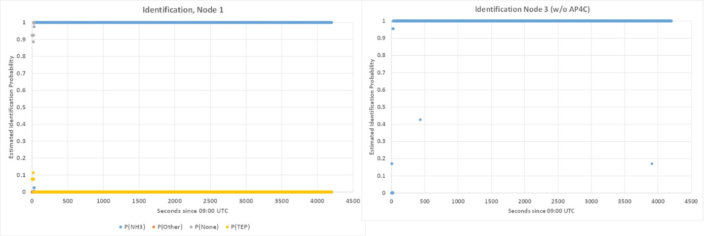
The controlled environment and the clean sensors almost certainly explain this perfect result. You should not expect such good results in all practical situations.
TNO Validation data set (17.12.2020)
This experiment was already referred to when discussing the performance of the anomaly detector. For additional information on anomaly detection and experimental setup, we refer to 4.1.1.2 Experimental Review of the anomaly detector (section: Anomaly detection caused by a real incident).
Figure 26 displays the results of the classification function for that test. This can be compared tithe timeline against Figure 11. The left plot is for Node 2 (exposed), the right plot is for Node 1 (not exposed). The colours indicate different classifications/substance classes. These are drawn semi-transparent, that is mixed colours correspond to situations where several classes have been identified.
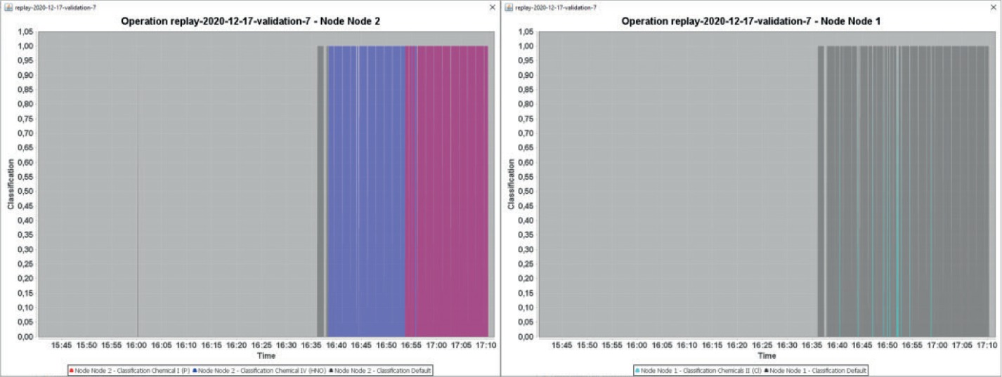
Grey is for the Default class, that is to say no other class could be identified. This naturally always stands alone since it indicates that no other substance class could be identified. Blue is for Chemicals IV (Nitrogen), Red is for Chemical I (Phosphorous), Cyan is for Chemicals II (Chlorine). At the times where both a NH3 and a TEP signal were applied, we have a mixed colour (dark magenta) superimposed by blue and red.
The short Grey peak early in the left graph corresponds to a short anomaly detected at that time on the MO-array. From approx. 16:38 onward the NH3 signal is detected as “Chemicals IV” and from approx. 16:53 also the TEP signal is detected as “Chemicals I” on Node 2.
Node 1 was not intentionally exposed. Nevertheless, anomalies were identified here as well as already explained in section 4.1.1.2. In contrast to Node 2 however, the classification almost always results in “Default”. There are some very short cyan peaks, which indicate a signal anomaly in the area of were usually Chlorine on either the IMS H2O or the IMS NH3 would be expected.
Additionally, the original dataset was processed using the same batch tools as the test from 23.11.2020 documented in the previous section. Figure 27 visualises the result of applying identification and the concentration estimation to data of Node 2. The small picture below the plots visualises the FPD raw data as a qualitative reference, which reflects the time development of the experiment (cyan – the HNO channel, responding to NH3; orange – the Phosphorous channel, responding to TEP).
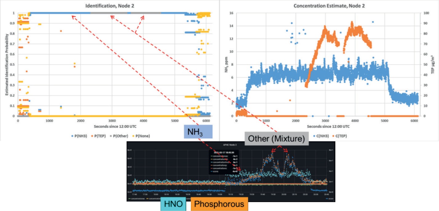
As soon as the NH3 signal pops up, the identification probability for NH3 goes to 1 and the concentration estimate increases. The actual absolute concentrations are not known to anybody but TNO, since this is a validation dataset. However, we assume that the base level concentration of NH3 is actually quite low. The noisy fluctuations of the concentration estimate are due to missing smoothing over time.
This situation does not change for a while until the TEP signal exceeds a certain level. Now, the identification jumps to “Other”! As already explained in 4.1.2.1, the reason for this is the construction of the Bayesian network that performs the identification. It assumes that the sensor is exposed to a single substance. Therefore, when detecting neither pure NH3 nor pure TEP, this contradicts the prior trained knowledge of the net. With that in mind, the output “Other” is completely correct. Nevertheless, this is not satisfactory of course. It would be possible to modify the network so that it is able to result in a list of probabilities of different substances, instead of being decisive for one substance (multiple simultaneous binary classifications).
The exposition of a mixture of substances in the validation experiment posed is a good stress test for the system. Moreover, it reveals that mixtures can be a general problem for chemical sensors: The NH3 in the sample massively influences the signal of the IMS H2O. TEP does not show the usual expected peak positions anymore. Instead, the peaks are shifted to positions comparable to the IMS, which has been doped with NH3.
This is an important example that the chemistry of a mixture in combination with the chemistry of the chemical sensor can literally lead to unpredictable effects. The best way to overcome this is probably to use as many sensors as possible and hope that most sensing technologies are not influenced too much by unwanted chemical side effects, thereby distorting the correct result.
Conclusions
The paper describes our work in the EU-SENSE project. The focus is on multi-sensor data fusion of chemical point sensors in a network developed in this project. The aim of data fusion was to improve the detection capabilities and the estimation of the concentration of the detected substance(s).
Detection is a classification task and improvement of detection means enhancing the discriminatory power of the classifier, that is to say reducing false alarms, false positives and false negatives. This was achieved by a two-step procedure. First, a sensitive anomaly detection identifies significant changes in the input stream of sensor responses by comparing the actual sensor response input (-vector) with the responses in a time-period in the past. This leads unavoidably to anomalies caused by harmless events. Therefore, in a second identification step, this anomaly has to be verified as a real incident. Mathematically, the fusion is achieved by means of statistical and Machine Learning methods. Bayesian networks proved to be useful, in particular when fusing information from multiple sensors.
Experiments carried out during the project, in order firstly to gather the necessary data and secondly to validate the developed approach, show that detection and concentration estimation works satisfactorily well. However, the set of substances to detect is very limited. It was not possible to build up a practically relevant substance library with many target substances within the project from scratch.
The sensors in the network are chemical point detectors, partially very sophisticated, mature but also costly. From an area coverage point of view, such a network is costly. Therefore, future work should consider whether standoff-detectors can be integrated in such a network and how their results can be fused.