Concerns on the issue of defence expenditure in the post-crisis Greece

The paper aims to tackle a controversial issue, namely the anticipated developments regarding defence expenditure once the Greek economy returns to growth. Such a comeback is expected to occur following a prolonged recessionary period during which defence spending cuts were a top priority, as recommended by the IMF, the ECB and the EC, members of the so-called “Troika”. The paper uses both conventional econometrics as well as neural networks to consider and evaluate the hierarchy’s ordering of the determinants used in such a demand for defence expenditure based on their explanatory power. While the role of property resources is certainly pronounced, as expected, human resources variables also seem to be able to explain defence spending developments, especially in the recent past. A forecasting investigation based on this background points to a number of interesting conclusions on the anticipated developments concerning defence spending in the future as well as on the determinants of such developments which might represent a threat to NATO cohesion.

Introduction

The issue concerning defence expenditure of Greece has been very popular in the literature considered both in the context of the country’s economic performance, as well as in an environment of an arms race against Turkey. The importance attributed to the question of the extent to which defence spending is excessive or not has led to a debate both in the scientific literature and the daily press following the economic crisis in Greece and its reluctance to abide by the repeated memoranda recipes suggested by the IMF, the ECB and the EC, members of the so-called “Troika,”¹ according to which defence procurement cuts have always been a top priority. The declared intention of the US presidency to revise the country’s contribution to NATO asking the allies to contribute more and avoid free-riding tactics has added to this debate, despite the fact that Greece seems to be one of the few allies that contribute a fair share in terms of NATO requirements². Given this background and in anticipation of the Greek economy returning to a path of growth after a long recessionary period, concerns have risen over the possibility that there will be more room for an increase in defence spending. Such an increase seems imperative, bearing in mind that the schedule of the procurement programmes of the Hellenic Armed Forces (EMPAE) has been repeatedly postponed during the crisis years, thus endangering their effectiveness³ in a period during which Turkey is threatening to ask for a revision of the status-quo in the Aegean and the Eastern Mediterranean.

This paper aims to look into this issue, namely the possibilities that the economic recovery of the Greek economy may offer more room for increased defence spending and the reasons that may trigger such an increase. The techniques of analysis employed use artificial intelligence and conventional methods, a combination that has proved to be very efficient in the past. Thus, following a brief literature review accompanied by the justification for using the neural networks technique, we proceed with a description of the input data and the methodology used in the analysis. Sections IV and V present the econometric results and the policy implications derived, while the final part of the paper draws conclusions.

A Brief Literature Review

The majority of the papers on the issue use conventional models for a time series or panel analysis employing three main variable categories: Economics and production, technology and geopolitical and security ones. Following a number of early, well-established contributions in the literature such as Smith (1980 and 1989), Hartley and Hooper (1990) Jones-Lee (1990) and Hewitt (1992), some focusing on developing countries e. g. (Deger and Smith 1983, Biswas and Ram 1986), there have been a number of papers concentrating on individual country cases (Murdoch and Sandler, 1985, Smith, 1990, Looney and Mehay, 1990) and alliances (Murdoch and Sandler, 1982, Knorr,1985, Okamura, 1991). The case of Greece occupies a leading position in the literature as it is involved in an arms race against Turkey (e. g. Sezgin, 2000, Andreou and Zombanakis 2006). Coming to recent contributions, there seems to be a trend which emphasises human resources and raises welfare considerations, some of them with reference to the Chinese case like Ying Zhang, Rui Wang and Dongqi Yao (2017), Ying Zhang, Xiaoxing Liu, Jiaxin Xu and Rui Wang (2017) and Fumitaka Furuoka, Mikio Oishi and Mohd Aminul Karim (2016). In fact, human resources variables like population growth and per capita income are considered as significant determinants (Dunne et al 2001, Dunne and Perlo-Freeman, 2003). Finally, on the techniques of analysis issue and following the inconclusive results derived on this issue using conventional models (Hartley and Sandler 1995, Taylor 1995, Brauer 2002), the focus has shifted towards artificial intelligence methods and specifically Artificial Neural Networks (ANN) to determine the defence expenditure of Greece (Andreou and Zombanakis 2000 and 2006).

ANN belongs to a class of data driven approaches, as opposed to model driven approaches most frequently used in the analysis. Some of the advantages of using ANN as have been analysed in the literature (Kuo and Reitch, 1995, Hill et al. 1996) are the following: First, they do not require any a - priory specification of the relationship between the variables involved in the relationship under consideration. Thus, in cases of disagreement on the issue of the explanatory variables to be used or in cases in which there is lack of a strong theoretical background, the ANN are considered to be preferable⁴ Quoting Beck et al. (2004), neural networks “can approximate any functional form suggested by the data, even if not specified by one’s theory ex ante”. In other words, neural networks are particularly suitable for a large number of defence-studies cases in which a standard theory cannot conclude as to a specific model structure or when immediate response to environmental changes is required. In addition, in cases in which certain variables are correlated or exhibit a non-linear pattern of behavior, the ANN are more applicable. This is due to the fact that ANN, being a data-science model, are not affected by statistical multicollinearity issues, while their non-linear nature enables better data fitting. Furthermore, without requiring the choice of a specific model, the network is designed to automatically perform the so-called estimation of input significance, as a result of which the most significant independent variables in the dataset are assigned high synapse (connection) weight values, while irrelevant variables are given lower weight values. It goes without saying that the choice and hierarchy of variables on the basis of input significance contributes to the forecasting performance of the network (Andreou and Zombanakis 2006). Finally, the use of ANN does not require any data distribution assumptions for the input data, which is a common issue when running a regression (Bahrammizaee, 2010). Finally, there is also evidence that neural networks display a higher forecasting ability when it comes to time series forecasting (T. Hill, et al. 1996, Adya, and Collopy 1998).

Input Data and methodology

The methodology that our paper follows is stepwise: First, we need to determine the forecasting ability of our neural network when it comes to the demand for defence expenditure in Greece and the leading input variables contributing to its forecasting performance. Given that the results of the input – significance procedure is derived on an ordinal, rather than a cardinal basis, our second step requires the use of Fully-Modified Ordinary Least Squares (FMOLS) to provide elasticity measures for the leading determinants of Greek defence expenditure as these have been selected by our ANN.

Input Data

The dataset used in this study contains the following variables as described in Table 1 and is composed of 57 observations covering a period between 1960 and 2016⁵.

Table 1

The Dataset

Code	Data Series	Source
EQDEF	Greece: Expenditure on Defence Equipment / GDP	NATO and SIPRI
SPILL	NATO Defence Expenditure / GDP	NATO and SIPRI
DLGDP	Rate of change of Greek GDP	ELSTAT
THREAT	Turkey: Expenditure on Defence Equipment / GDP	NATO and SIPRI
DRPOP	Turkey-Greece: Difference of Population Growth Rate	UN STATISTICS

Methodology: The Use OF ANNs

The neural network model has been estimated through the Keras Python library (Chollet et al., 2015). We used several alternative configuration schemes when it came to the number of hidden layers and the neurons in each hidden layer. Through this process, we were able to achieve performance and also compare how the different network architectures perform on this dataset. The input and output data series are normalised in the range [0,1], while the learning rate and momentum coefficient were fixed at 0.001 and 0.9 respectively. We also utilised the Nesterov momentum since it helps significantly in the process of searching for a local minimum. Regarding the activation functions, we used ReLu for the neurons in the hidden layers and Sigmoid for the neuron in the output layer.

Each input variable is associated with one neuron in the input layer. The frequency of the data is annual and the observations are split to 80% in-sample / training and 20% out-of-sample / testing. Determining the number of hidden layers and neurons in each layer is a difficult task and it plays a highly significant role in the performance of the model. If a hidden layer contains too few neurons, a bias will be produced due to the constraint of the function space which will result in poor performance. On the other hand, if too many neurons are used, overfitting might be caused and the amount of time needed by the model to analyse the data will increase significantly, which will not necessarily lead to convergence. We therefore tested the model performance of various combinations of hidden layers and neurons in each hidden layer, in order to obtain the best forecasting performance.

The number of iterations/epochs that present the data to the model also play a significant role during the training phase. We try different values of epochs in our models to investigate which leads to the highest accuracy. The number of epochs that were tested in each case ranged between 3,000 and 15,000. However, it should be mentioned that a large number of epochs might cause overfitting and the model will not be able to generalise.

The issue of overfitting can be overcome by evaluating the out-of-sample forecast performance of the model through the usage of a testing set. The testing set contains unseen parameters that were not included in the dataset during the training phase (Azoff, 1994). If the network learned the structure of the input data instead of memorising it, it performs well during the testing phase. On the other hand, if the model did memorise the data, then it will perform poorly on the out-of-sample forecast. Therefore, the optimal network architecture is generally based on the performance of the out-of-sample forecast, assuming that the learning ability was satisfactory.

The out-of-sample forecast performance is evaluated using three different types of forecast evaluation statistics. The evaluation statistics used are the Root Mean Squared Error (RMSE), Mean Absolute Error (MAE), Mean Absolute Percentage Error (MAPE), and the Theil Inequality Coefficient (Theil’s-U). We employ various evaluation statistics since there are certain similarities and differences in each error statistic. To be more specific, all error statistics overcome the cancellation of positive and negative errors during their summation; however, they do not take into consideration the scale of the series that is tested, while the MAPE and Theil’s-U do. It should be mentioned that for small errors, the MAPE is bounded between 0% and 100%, but for large errors there are is no upper boundary, while in the case of Theil’s-U, the series is always bounded between 0 and 1. When comparing the MAPE, one looks to see if the value of the MAPE is less than 100%, while in the case of Theil’s-U, it is of interest to see whether the error statistic is as low as possible.

RMSE=1T∑t=1T(xtf−xt)2

MAE=1T∑t=1Txtf−xt

MAPE=100T∑t=1Txtf−xtxt

Theil's U=1T∑t=1T(xtf−xt)21T∑t=1T(xtf)2+1T∑t=1T(xt)2

where is the forecast value, xt is the actual value when pattern t is presented and T is the xtf total number of observations.

Methodology: The use of Conventional techniques

Turning to using conventional analysis and following Smith (1989), we shall assume that the demand for defence expenditure is represented as follows⁶.

DEF = fY, P, S 1

where DEF is a specific country’s defence spending depending on income (Y), prices of defence and civilian goods (P) and selected geopolitical variables depending on the country in focus (S). Given the controversial role of prices in the equation as earlier pointed out, (Sandler and Hartley 1995), prices are usually not included as an explanatory variable and the demand for defence expenditure in its general form reduces to:

DEF = fY, S 1’

In the case of Greece, following Andreou at al. (2002), we expand (1’) to get the following generalised formulation:

EQDEF= fDLGDP,DRPOP,SPILL,THREAT,Z 2

where EQDEF stands for GDP share of defence expenditure on equipment procurement, DLGDP is the country’s GDP rate of growth, SPILL stands for the spill over benefits as these are denoted by the defence spending over NATO – GDP figures and DRPOP represents the difference of the population growth rates between Turkey and Greece. The choice of the DRPOP has been based on the emphasis on the human resources variables (Andreou and Zombanakis 2000 and 2011) in a period in which the Turkish side has explicitly underlined its importance⁷. The four-year lag of the dependent variable is used to represent the follow-up of the Hellenic Armed Forces armaments programme (EMPAE), as this is strongly affected by the political cycle⁸. Concerning Z, this has been reserved for dummies capturing various extraordinary major geopolitical and economic interventions taking place in this half-century period like the oil shock and the financing of the Olympic Games (DUMMYECON) and the repeated elections especially during the memoranda period (DUMMYPOL).

The final variable used in the model is THREAT, representing the Turkish GDP share of expenditure on equipment procurement and approximates the pressure exercised on Greece by Turkey. This pressure has already been ongoing since the beginning of the 50s, but has been culminating during the last two decades, with the Turkish president demanding revision of the Lausanne Treaty of 1923 and the Paris Treaty 1947, which describe the status quo of the Greek islands in the Aegean, during his visit to Athens on December 6, 2017.

Results

ANN out- of – Sample Forecasting

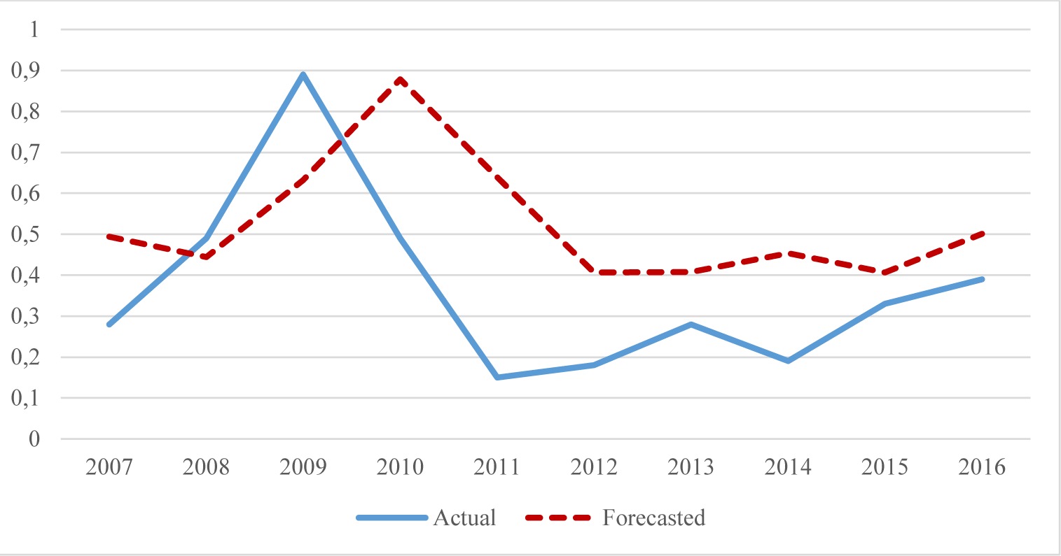
Table 2 shows the out-of-sample forecast evaluation statistics of the various neural network architectures. It can be observed that despite the limited number of observations, the neural network predicts the movements of the series to a quite significant extent. The best forecast is given by the neural network architecture of 5-10-10-1 with 15,000 epochs. To be more specific, the best forecast has an RMSE of 0.237, MAE of 8.203, MAPE of 68.417% and a Theil’s-U of 0.262. It is important to note that the MAPE is below 100% and the Theil’s-U value is significantly less than 1. We also include a graph of the best forecast made by the optimal neural network architecture (Figure 1).

Table 2

Neural Network Out-of-Sample Errors

Neural Network Training Output
Epochs	Network Architecture	RMSE	MAE	MAPE	Theil’s-U
3,000	5-5-1	0.310717	23.5922	117.7867	0.30062
5,000	5-5-1	0.294317	21.66696	110.3888	0.289692
6,000	5-5-1	0.285677	20.53927	105.9668	0.283892
10,000	5-5-1	0.259369	16.06252	90.00123	0.267201
15,000	5-5-1	0.246835	12.66605	80.90017	0.261674
15,000	5-10-1	0.241798	12.32441	76.62717	0.256324
15,000	5-15-1	0.248351	14.82829	82.11732	0.257223
15,000	5-10-10-1	0.237731	8.203952	68.4175	0.261517
15,000	5-10-15-1	0.243964	10.61792	74.89064	0.262506
15,000	5-10-10-10-1	0.241384	8.918298	70.0614	0.263523

Figure 1

Actual and Forecast Values of Equipment Defence Spending

https://securityanddefence.pl/f/fulltexts/103408/SDQ-24-177-g001_min.jpg

Determining the Input Significance

An important aspect of our study is the determination of the significance ordering of the input variables. To be more specific, the input variables that are most significant are those that contribute mostly to the forecasting process. This process is also carried out in Andreou and Zombanakis (2000) study and is explained extensively in Azoff (1994). The significance of the input variables is determined through the sum of the absolute values of the weights fanning from each input variable into all the nodes in the first hidden layer. The input variables that have the highest connection strength are the ones that contribute significantly to the forecasting process. The analytical technical background behind this process is beyond the scope of our study, since the reader may refer to Azoff (1994) for further information.

The training phase of the model includes 45 annual observations and covers the period 1960-2006, while the testing phase contains 12 annual observations and is from 2007-2016. The input significance ordering of the variables used in forecasting the equipment defence of Greece is an important part of our study. The reason is because not only does it show which variable contributes mostly to the forecasting of the variable of interest, but also because inferences can be made on the ordering of the variables that mostly affect the equipment defence spending of Greece.

As stated earlier, the input significance ordering is obtained through the summation of the absolute values of the weights of each input to the neurons of the first hidden layer. Once this process is complete, we rank the variables in descending order to obtain a clear picture of the most significant variables. The results are presented in Table 3 where W denotes the weight of each variable that appears as a subscript.

Table 3

Ordering of Neural Network Weights

Estimation of Input Significance
W_threat>W_dlgdp>W_drpop>W_spill

According to the optimal forecast generated by the neural network architecture of 5-10-10-1, the input significance ordering is W_threat>W_dlgdp>W_drpop>W_spill. It is interesting to see that Turkish defence spending on equipment ranks first in terms of input significance ordering as a determinant of Greek defence equipment procurement, followed by the GDP growth rate and the variable denoting demographic developments. The spill-over benefits accrued due to the country’s NATO membership do not seem to be a decisive determinant possibly reflecting the reliability of NATO support as this is assessed by the authorities⁹. This hierarchy ordering is very helpful and we shall come back to it once we have concluded a FMOLS estimate, which will be used to complement our ANN findings so far.

Adding to the Results Using FMOLS

Using the data set as described above and transforming the variables in logarithmic form the specification of equation (2) leads to the following estimate:

LEQDEF = c1*DLGDP+c2*DRPOP + c3*LSPILL+ c4*LTHREATc5*LEQDEF−4 + c6*DUMMYECON +c7*DUMMYPOL + C8 3

All variables, except for DLGDP, are I(1) so, we are concerned about the possibility of a spurious regression. Furthermore, assuming that the regression is co-integrated, OLS will be consistent, (actually super consistent) but parameter estimates might suffer from small sample variance. The underlying dynamics are absorbed by the error term, which might result in heteroskasticity and / or autocorrelation. Following standard practices, the equations are estimated by FMOLS and, of course, we test for co-integration. It turns out that the equation as depicted in table 4 is co-integrated, residuals are normally distributed and there is no evidence of autocorrelation. Parameter estimates are all significant and bear the expected signs, thus supporting the theoretical background discussed above.

Table 4

Parameter Estimates for Eq. (3)

Dependent Variable: LEQDEF
Variable	Coefficient	Std. Error	t-Statistic	prob.
DLGDP	2.412603	0.632180	3.816321	0.0004
DRPOP(-4)	27.19353	12.74381	2.133862	0.0387
LSPILL	0.896752	0.194348	4.614150	0.0000
LTHREAT	0.633856	0.076954	8.236833	0.0000
LEQDEF(-4)	0.362379	0.093196	3.888337	0.0004
DUMMYECON	–1.165697	0.137698	–8.465628	0.0000
DUMMYPOL	0.752575	0.128696	5.847711	0.0000
C	–1.684792	0.209687	–8.034776	0.0000
R-squared	0.762995	Mean dependent var		–0.609395
Adjusted R-squared	0.723495	S.D. dependent var		0.535097
S.E. of regression	0.281374	Sum squared resid		3.325203

Finally, in order to assess the relative importance of the regressors, it was decided to estimate the model using a stepwise regression treating LEQDEF (-4) and the two dummies as fixed regressors. The estimation process is reported in Appendix II and suggests an input significance ordering as depicted in table 5 below, in which it is compared to that derived using ANN.

Table 5

Input Significance Ordering by Estimation Method

Variables Ranking	ANN	STEPWISE
1	THREAT	DRPOP
2	DLGDP	THREAT
3	DRPOP	SPILL
4	SPILL	DLGDP

Policy Implications and Forecasting

Table 5 sums up the results of the input-significance ordering procedure using both ANN and a stepwise regression. It is evident that THREAT which is approximated by the Turkish defence spending on equipment features in one of the two top positions in both rankings. On the human resources side, another variable related to Turkey, namely DRPOP, which stands for the difference in population growth between Turkey and Greece, is at the top of the FMOLS hierarchy order. Both the dependent variable and the one denoting population growth differences enter the right-hand side of the equation with a significant time lag. In the case of the latter and due to the long-run nature of the demographic problems in general, the lag accounts for the series of recognition, administrative, operational and effectiveness lags involved in the implementation of the appropriate policies. In the case of the defence equipment procurement, a four-year time lag has been considered as representing the political cycle which usually reflects the changes of governmental priorities concerning this sensitive issue¹⁰. In contrast to THREAT, the SPILL variable appear to rank at the bottom of the input-significance ordering due to the reasons discussed above, with everything that this may entail concerning its implications on the issue of NATO cohesion.

It is expected that the first determinant to be focused on, despite its low ranking in the stepwise input-significance ordering, must be the GDP, given the repeated worries about a possible increase in defence spending once the economy returns to a growth path (IMF, 2010, 2012, 2014). The elasticity estimate given in Table 4 indicates a pronounced response of the defence procurement to the expected increase. It must be taken into account, however, that this response does not mean that the entire GDP rise is going to be devoted to defence spending, given that the percentage of the GDP channeled to defence equipment procurement has been fluctuating between 0.15 and 0.39 over the past few years. Thus, one can safely argue that even such elastic behaviour is not expected to lead to percentages higher than 0.4 of the GDP given to equipment defence expenditure in the next few years following a GDP rise of the order of 2% (Ministry of Finance 2017).

Going into the matter further and examining the extent to which such behaviour has been uniform throughout the period under consideration, we considered the possibility of a break in the series by running the OLS with breakpoints for the GDP variable. It turned out, however, that such an experiment yielded no breakpoints, meaning that the elasticity computed is the same throughout the period under study. Still, an additional point of investigation would argue a difference in elasticity depending on the extent to which the GDP has been increasing or decreasing during the time range considered. To look into the matter, we used a modified version of (3) in which the DLGDP variable is broken into two coordinates depending on the extent to which it has been positive or negative. The resulting elasticity coefficients indicate that spending on defence equipment is not sensitive to GDP increases unlike the case of GDP reductions, in which case it tends to rise aiming at retaining an ‘”acceptable” defence spending fraction of the GDP¹¹.

Turning to the Turkish defence expenditure represented by THREAT in the equation, its predominance in the ordering of input significance deserves special attention in this case and focusing on it has led to the following findings:

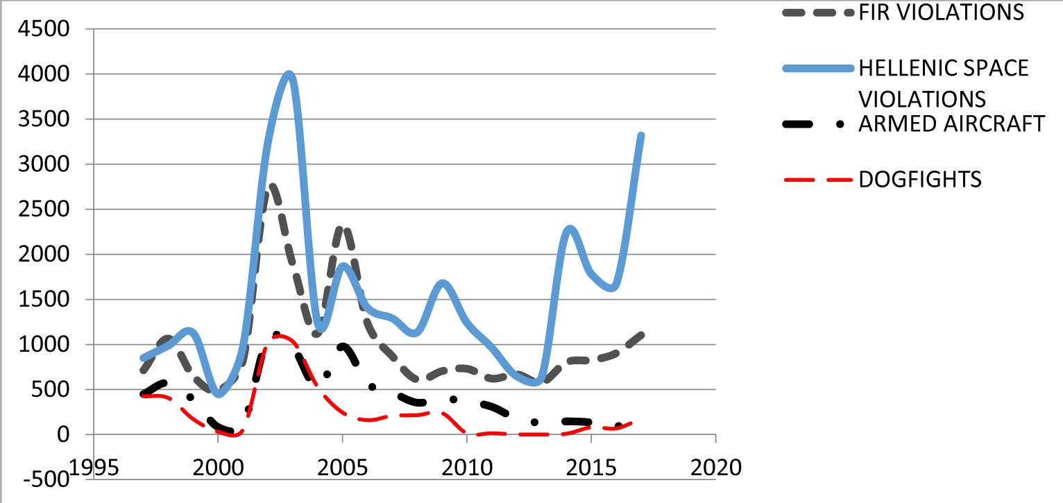
Running an OLS with breakpoints shows that the only determinant exhibiting a break with regard to its effect on the dependent variable is THREAT. More specifically, the Greek equipment procurement was strongly inelastic (0.21) before 2003 shortly after the AKP rise to power¹². After that year, the picture changes dramatically, with the behaviour becoming elastic (1.32) given that the pressure exercised on the part of Turkey rises (see Table A. III. 1 in Appendix III and Figure 2 below). Figure 2, in particular, shows how the Turkish Airforce’s (THK) hostile activity expressed as Hellenic Air Space and FIR violations, armed aircraft and engagements (dogfights) in the Hellenic airspace reached an overall maximum during that specific year¹³.

Figure 2

THK Activity in the Hellenic Airspace

Source: HAF, NATO.

https://securityanddefence.pl/f/fulltexts/103408/SDQ-24-177-g002_min.jpg

We then proceeded with modifying equation (3) to account for increases or decreases of the THREAT variable as follows:

LEQDEF = c1*DLGDP +c2*DRPOP+ c3*LSPILL +c4*LTHREAT*THREATP +c5*LTHREAT*THREATN + c6*LEQDEF−4 + c7*DUMMYECON + c8*DUMMYPOL +C9 3’

As indicated in Appendix II, Greek defence expenditure reacts, almost symmetrically to increases and decreases of Turkish expenditure. The hypothesis of symmetric adjustment implies that c (4) = c (5), a hypothesis that can be tested via a Wald test. The results of the Wald test clearly indicate that the hypothesis cannot be rejected at conventional levels of confidence, which means that we can use (3) rather than (3’) without loss of generality. Indeed, the long-run elasticity estimate of the THREAT variable is unity, a fact that points to a well-balanced action-reaction process typical of an arms race environment¹⁴.

To conclude the section of policy implications, we thought that it would be appropriate to embark on a forecasting exercise based on the estimates of equation (3) for a medium and long-term outlook. The values assumed by the explanatory variables have been input as follows: The GDP growth rate for this period has been the one provided by the Mid-Term Fiscal Strategy Framework presented in the Greek parliament at the end of last year (Ministry of Finance 2017). The THREAT figures are based on the provisions of the $150 billion long-term (2000-2025) procurement programme of the Turkish armed forces¹⁵, while the DRPOP figures retain the current year growth rate for the forecast period.

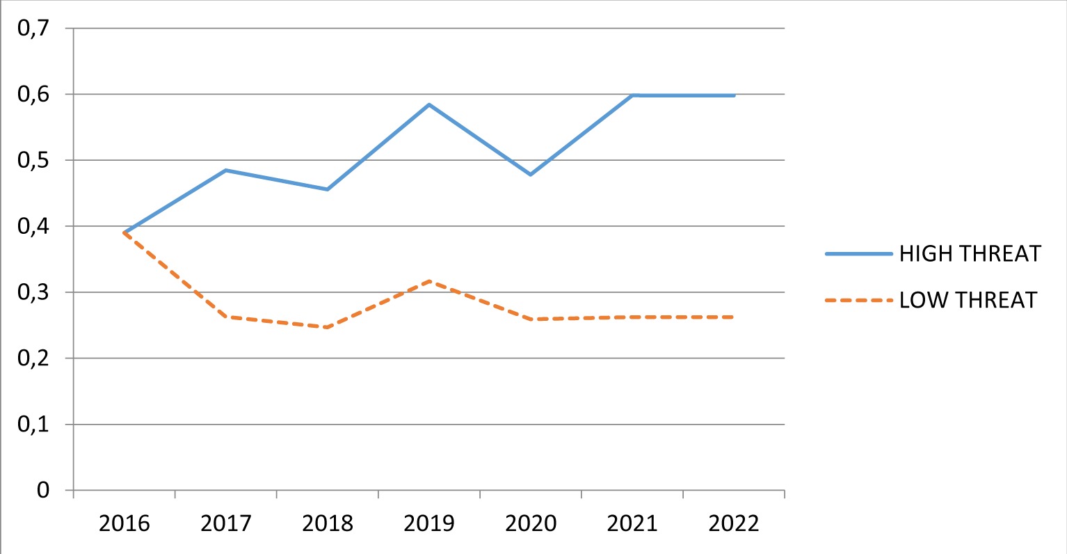
To underline the impact of a Turkish escalation policy on the Greek defence burden, we have tried an alternative option according to which the Turkish defence procurement assumes rather conservative values approximating the ones at the beginning of the 80s following the military coup. The results of both forecasting exercises are shown in Table 6 and Figure 3 below, with the first column denoting the Greek procurement as a response to Turkish escalation policies as these are currently manifested and the second showing the corresponding Greek figures for a conservative Turkish procurement policy. The impact of such a difference in the THREAT variable on the Greek side is impressive, as the figures of the third column are GDP shares equivalent to purchasing one extra latest technology HDW Type 214 submarine every year, or, alternatively, 25 Lockheed-Martin F-16 Block 52 aircraft, or even 80 KMW Leopard HEL-2 tanks!

Table 6

Hellenic Defence Procurement Responses to THREAT (Forecasts GDP Shares)

Year	Eqdef : Escalating Turkish Policy	Eqdef : Conservative Turkish Policy	Difference
2017	0,484836	0,26264	0,2222
2018	0,455764	0,246892	0,2088
2019	0,584243	0,31649	0,2677
2020	0,478078	0,25898	0,2191
2021	0,597934	0,262512	0,3354
2022	0,597988	0,262536	0,3354

Figure 3

Hellenic Defence Procurement Responses to THREAT (Forecasts GDP Shares)

https://securityanddefence.pl/f/fulltexts/103408/SDQ-24-177-g003_min.jpg

Conclusions

The aim of this paper has been to investigate the possibility of increased defence expenditure by Greece once the country’s economy recovers from the ongoing crisis, a move which is against the Troika policy recommendations. The results derived point to a number of interesting conclusions: First, the forecast shows that there will be an increase in defence expenditure on equipment procurement in the next few years.

Second, a return to positive growth rates is expected to bring about rather low, if any at all, increases as regards defence spending on equipment.

Third, the only source of such increases in the future is the corresponding expenditure of Turkey, in the logic of an arms race environment which has been threatening the NATO cohesion ever since 1974, when Greece had withdrawn from the alliance military structure for a period of six years. Such an environment accentuates the already existing frictions between Turkey and a number of the remaining NATO members for a wide selection of reasons.

Fourth, the pressure exercised in such an environment by Turkey has increased since the beginning of last decade, making the follow-up cost considerably heavy for Greece to sustain.

Acknowledgement: The authors wish to thank Professor Keith Hartley, Economics Department, University of York, as well as Major George Reklites, Hellenic Air Force for valuable contributions and comments.

Appendix I. NN Briefing

Artificial Neural Networks, which belong to the data science approach and not to the model driven approach, are one of the widely used models for data science applications. They are loosely based on the biological nervous system and brain functions, meaning that they employ certain general purpose algorithms to analyse the input data provided. The structure of an Artificial Neural Network contains the input layer, the hidden layers and the output layer. Each layer contains several nodes or neurons. Each neuron connection is assigned a weight that is based on its relative importance compared to the other inputs. The calculation of the weights that creates the input-output mapping are what solve the high dimensional, non-linear system identification problem. However, the model adjusts its weights in order to minimise the errors in the results. A commonly used process for the training is back-propagation, which is technically the derivative of the errors with respect to the weights . An example of an m-d-q neural network architecture is displayed in Figure 2 where m are the inputs, d are the number of neurons in the hidden layer, and q are the output neurons. In our study, we estimate an m-d-1 network architecture to forecast the behaviour of our time series.

Figure 4

Example of a Neural Network Diagram

https://securityanddefence.pl/f/fulltexts/103408/SDQ-24-177-g004_min.jpg

The input data is analysed by the neurons inside the hidden layers through the utilisation of activation functions such as Sigmoid and ReLu. (Hahnloser et al. 2000) The mathematical form of the Artificial Neural Network is presented below:

yt= wo+ ∑j=1qwj×g w0j+∑i=1pwij × yt−1+ ϵt

where wij(i=0,1,2,...,p'j=1,2,..q) and wj(j=0,1,2,..q) are the connection weights/biases, is the number of input neurons q and is the number of the hidden nodes. The output of the model yt is and the input variables which are the previous values are y_t-1. The error term is εt which is the difference in the forecast and actual values of the output and g is the activation function of the model. It should be mentioned that a commonly used parameter by artificial neural networks is the bias factor that has a fixed input value of 1 and it feeds into all neurons in the hidden and output layers with adjustable weights. Its significance is that it shifts the activation function which results in an increase in the accuracy of the data.

System Design

The input data, x=x(t):1≤t≤N is split into a training set x=x(t):1≤t≤T and a testing set x=x(t):T≤t≤N, where N is the length of the series. The training set is used to train the network at a certain level to achieve convergence based on some error criterion. This is achieved by presenting the input and output data L-times to the model and have the learning algorithm adjust its weights. The number of times that the data is presented are called epochs and the output neuron is basically the predicted values that the model predicts. The process of back-propagation is carried out by an optimiser such as Stochastic Gradient Descent (SGD) (Bottou, 2010). The momentum term (Qian, 1999) of SGD helps in accelerating the process by allowing the SGD to navigate better in ravines. However, although the momentum term has proved extremely useful, there has been an improvement on it which is known as Nesterov Accelerated Gradient (NAG) (Botev et al, 2017). This allows the calculation of the gradient not based on the current parameters but based on the future position of the parameters. In simpler terms, what NAG contributes to the process of searching for a local minimum is to move faster towards the local minimum when the slope is decreasing but move slower when the slope increases. Thus, a correction is made every time the new accumulated gradient is computed. The range of predicted values is between [0,1] by the implementation tool used. Therefore, the values xt of both the training and testing set is normalized by taking the ratio xtxmax−xmin, in order to avoid negative values. The predicted values can be restored by taking the inverse transformation xtf*(xmax−xmin).

Appendix II. The Conventional techniques of analysis results

Table A II.1.

Stepwise Regression of (3)

Dependent Variable: LEQDEF
Method: Stepwise Regression
Variable		Coefficient	Std. Error	t-Statistic	Prob.*
C		–1.684851	0.230026	–7.324621	0.0000
LEQDEF(-4)		0.342816	0.102247	3.352819	0.0017
DUMMYECON		–1.052857	0.151140	–6.966088	0.0000
DUMMYPOL		0.714025	0.140554	5.080084	0.0000
DRPOP(-4)		25.30914	13.98592	1.809616	0.0773
LTHREAT	0.625008		0.082260	7.597947		0.0000
LSPILL	0.894941		0.213277	4.196141		0.0001
DLGDP	2.190140		0.693677	3.157288		0.0029
R–squared	0.769931		Mean dependent var			–0.617479
Adjusted R–squared	0.732478		S.D. dependent var			0.532855
S.E. of regression	0.275606		Akaike info criterion			0.403414
Sum squared resid	3.266234		Schwarz criterion			0.706446
Log likelihood	–2.287068		Hannan–Quinn criter.			0.519212
F–statistic	20.55719		Durbin–Watson stat			1.695384
Prob(F–statistic)	0.000000
	Selection Summary
Added DRPOP(-4)
Added LTHREAT
Added LSPILL
Added DLGDP

Table A II.2.

Regression of (3) with Breakpoints

Dependent Variable: LEQDEF
Method: Least Squares with Breaks
Variable	Coefficient	Std. Error	t-Statistic	Prob.
1966 - 2003 -- 38 obs
LTHREAT	0.210782	0.078480	2.685790	0.0098
2004 - 2022 -- 19 obs
LTHREAT	1.317714	0.190273	6.925396	0.0000
Non-Breaking Variables
LSPILL	–0.474144	0.139625	–3.395837	0.0014
LEQDEF(-4)	0.260066	0.118229	2.199686	0.0326
DLGDP	1.008563	0.914584	1.102756	0.2755
DRPOP(-4)	35.08685	14.66667	2.392284	0.0206
DUMMYPOL	0.490865	0.164422	2.985401	0.0044
DUMMYECON	–0.972008	0.183594	–5.294343	0.0000
R-squared	0.703491	Mean dependent var		–0.706536
Adjusted R-squared	0.661132	S.D. dependent var		0.574195
S.E. of regression	0.334253	Akaike info criterion		0.775631
Sum squared resid	5.474512	Schwarz criterion		1.062375
Log likelihood	–14.10548	Hannan-Quinn criter.		0.887069
Durbin-Watson stat	1.008325

Table A II.3.

Parameter estimates of Equation (3’)

Method: Fully Modified Least Squares (FMOLS)
Variable	Coefficient	Std. Error	t-Statistic	Prob.
DLGDP	2.498464	0.643276	3.883970	0.0004
DRPOP(-4)	26.71190	12.91114	2.068903	0.0449
LSPILL	0.949501	0.199890	4.750122	0.0000
LTHREAT*THREATP	0.713434	0.089629	7.959886	0.0000
LTHREAT*THREATN	0.574822	0.089634	6.413015	0.0000
LEQDEF(-4)	0.359910	0.094415	3.811982	0.0005
DUMMYECON	–1.174320	0.139498	–8.418188	0.0000
DUMMYPOL	0.737484	0.130943	5.632096	0.0000
C	–1.750609	0.218007	–8.030068	0.0000
R-squared	0.768891	Mean dependent var	–0.609395
Adjusted R-squared	0.723797	S.D. dependent var	0.535097
S.E. of regression	0.281220	Sum squared resid	3.242481
Long-run variance	0.064683

Table A II. 4.

Wald test for equation (3’) testing c(4) = c(5)

Wald Test:
Equation: (3’)
Test Statistic	Value	df	Probability
t-statistic	1.566997	41	0.1248
F-statistic	2.455479	(1, 41)	0.1248
Chi-square	2.455479	1	0.1171
Null Hypothesis: C(4)=C(5)
Null Hypothesis Summary:
Normalized Restriction (= 0)		Value	Std. Err.
C(4) - C(5)		0.138612	0.088457

Appendix III. The Greek / turkish arms race in figures

Table A III. 1.

Turkish Air Force Activity in the Hellenic FIR

Year	Fir Violations	Hellenic Space Violations	Armed Aircraft	Dogfights
1997	712	849	448	425
1998	1064	986	574	405
1999	648	1125	384	171
2000	487	446	82	30
2001	826	976	105	53
2002	2742	3240	1062	1017
2003	1891	3938	970	1032
2004	1121	1241	521	528
2005	2330	1866	977	244
2006	1237	1406	567	159
2007	868	1289	464	207
2008	608	1134	353	215
2009	703	1678	395	237
2010	729	1239	367	13
2011	620	962	307	13
2012	667	646	176	1
2013	577	636	129	0
2014	801	2244	145	8
2015	826	1779	133	80
2016	902	1671	86	68

Source: Hellenic General Staff

FOOTNOTES

1 Popular term widely used in Greece, Cyprus, Ireland, Portugal and Spain to refer to the presence of the International Monetary Fund, the European Central Bank and the European Commission in these countries since 2010 and the economic policy measures that these institutions have proposed and monitored in order to deal with the economic problems arising in each case.

2 In fact there is more to this issue than what meets the eye (Ragies, 2017): Indeed, during the recent NATO summit in July, it has been pointed out that only five allies (US, UK, Poland, Greece and Estonia) contribute 2% or more of their GDP to defence. The fact remains, however, that regarding Greece, roughly 70% of its defence spending represents inelastic spending on salaries, wages and pensions of military and civilian personnel and only about 25% to equipment and infrastructure spending, which includes contributions to the alliance such as the NMIOTC (NATO Maritime Interdiction Operational Training Centre) in Crete.

3 Acronym in Greek for the Long Term Programme for the Development and Upgrading of the Armed Forces, In fact the IMF has repeatedly expressed its concerns on the issue of “excessive defence spending” in the past (IMF, 2010, 2012 and 2014).

4 In the case of the demand for defence spending, for example, the use of prices as an explanatory variable is an open issue (Sandler and Hartley 1995).

5 The theoretical background behind the selection of these variables is provided below.

6 This model is derived by using a social welfare function which is maximised subject to a number of constraints; both budgetary and geostrategic ones (see Smith, 1980, 1989, for further details).

7 In fact, during his speech in Eskişehir, in March 2017, the Turkish president urged “his brothers and sisters in Europe” to “have not just three but five children,” thus beginning a baby boom in their new countries.

8 The effect of the political cycle is especially pronounced when it comes to recording transactions on importing defence equipment. Depending on whether the recording system is based on accruals or payments, the political cost involved in terms of a “guns versus butter” logic dilemma will burden the ruling party during the period under consideration.

9 The NATO support has been questioned since 1974 and the Turkish invasion to Cyprus, following which Greece withdrew from the NATO military structure for a period of six years.

10 On the decisive role of politics in this issue consult Hartley (2012).

11 Retaining an “acceptable” defence equipment ratio between Greece and Turkey has always been subject to rules going back to the decades of the 60s and 70s with an analogy of 7/10 for the US FMS programmes supporting the armed forces of these two NATO member countries.

12 AKP stands for Justice and Development Party.

13 The emphasis given to FIR and ICAO violations at the expense of engagements during the last few years may be due to the fact that a large number of experienced pilots have left the THK following the July 2016 coup attempt. In addition, recent experience indicates a shift to alternative forms of aggression involving mainly naval tactics. Thus, on February 12, 2017 a Turkish coast guard vessel rammed a Greek one while performing what the Greek coast guard called “dangerous manoeuvres inconsistent with international collision avoidance practices.” The fact that the incident took place near Imia, a pair of Greek islets the ownership of which Turkey has disputed for 20 years, points to territorial power play. The threat mix involves, in addition, certain rather unorthodox methods like the arrest of two Greek Army officers during a border patrol in the north on February 28 and their imprisonment since then without any charges being pressed.

14 It has now been established in the literature that the Greek side is compelled to follow the Turkish defence procurement policy regardless of its direction of change and refers to earlier work on this issue (Andreou and Zombanakis 2000, 2006 and 2011) in which an arms race between the two sides has been established. The fact is, however, that the defence potential of Turkey has risen despite its recent economic problems, with the government even aiming to purchase F-35 stealth fighters for $100 million each. By contrast, the ability of Greece to build up a reliable defence industrial base will be eroded without new investments.

15 The recent purchase of the Russian S-400 ground to air missiles from Turkey for about $2.5 billion, a system outside the NATO umbrella, seems to be over and above these long-term procurement programme provisions. The cost will be covered partly by a loan from Russia denominated in rubles. The fact remains, however, that such moves tend to threaten the NATO cohesion over and above the Greek-Turkish friction, following the tense relations with a number of NATO members over e. g. the Turkish rapprochement with Russia and Iran, the EU-Turkish relationship, the US support to the Kurds and the refugee issue.

REFERENCES (43)

Adya, M. and Collopy F, 1998. How Effective are Neural Networks at Forecasting and Prediction? A Review and Evaluation, Journal of Forecasting, 17 (5-6), pp. 481-495. doi: 10.1002/(SICI)1099-131X(1998090)17:5/6<481::AID-FOR709>3.0.CO;2-Q.

eISSN:	2544-994X
ISSN:	2300-8741