Introduction

During the EU Summit in Versailles in early March 2022, a proposal was put forward that defence expenditure should not be included in the annual fiscal budgets and, consequently, in the national debt of EU member countries. Since then, there has been extensive discussion in the media on the degree to which defence spending burdens the national debt. Bearing in mind that some member countries have expressed scepticism about such proposals, it may be constructive to take a fresh look at the military debt issue, given the current geopolitical and economic developments.

Greece, like some other EU member countries, has recently embarked on a substantial defence procurement programme to strengthen its national defence capabilities despite its tight fiscal conditions (see Table A2 in the Appendix). The decision has developed into a controversial issue and raised concerns regarding the fiscal impact of such a considerable purchase during a period characterised by serious financial constraints. The purpose of this paper is to take a close look at the various defence equipment procurement programmes and how these have affected the national debt of Greece since the beginning of the eighties. To do so, we devote special attention to the determinants of the military debt of the country via a specific equation which accompanies the one that determines the national debt. Thus, the novelty and, consequently, the contribution of the paper is that using the system of these two equations it focuses on the interaction of the military debt and the national debt of Greece, with the former being a variable which has never before been introduced in such analysis. We also introduce defence spending on equipment rather than the total defence expenditure variable for reasons extensively analysed later on in the paper. Finally, we argue that given the non-linear response of the public debt to increases in the military debt, the resulting burden diminishes overtime and tends to become negligible in the long run following prolonged payments schedules.

Background Information

To offer a first glance at the Hellenic Armed Forces defence procurement programmes, Table A1 in the Appendix shows the main purchases of heavy defence equipment between 1980 and 2004. These amount to a total value of about 10€ billion and indicate that assuming an even distribution of the corresponding flow of payments during the period in question, the average annual spending is about 450€ million or 0.5% of the GDP, or 0.6% of the total public debt of the country during that period. In terms of payment procedures, however, beginning in 1995, the debt of the armed forces was reduced to zero following a change to the recording philosophy. According to this, defence expenditure on equipment is considered as fixed capital formation, i.e. investment flows rather than intermediate expenditure (EU, 2013). This means that the flow of payments regarding armed forces equipment purchases has been arranged to follow a pattern of long-term credits related to transactions between the Hellenic Republic and the contractor, or contractor’s government (G to G), in each case. These are regarded as loans equal to the amount required to finance each programme and signed for the total amount of the programme under consideration. The payment flows, however, take the form of annual instalments or long-term credit servicing of each loan, extending to a considerable number of years following the procurement date. This means that the annual budget is burdened for the instalment paid every year and not by the total value of the equipment purchased. Given the confidentiality of the detailed specifications of the various defence - procurement - programme figures, the only source of information is the relevant payments made for each programme recorded in the form of down payments, which are not included in the external debt figures (EU, 2013). Following the change from payments to accrual basis recording of defence equipment procurement by the Eurostat - ESA¹ in 2005 and the subsequent problems facing the Greek economy, defence equipment purchases were brought to a standstill from 2009 onwards, while all pending payments were concluded by 2015.

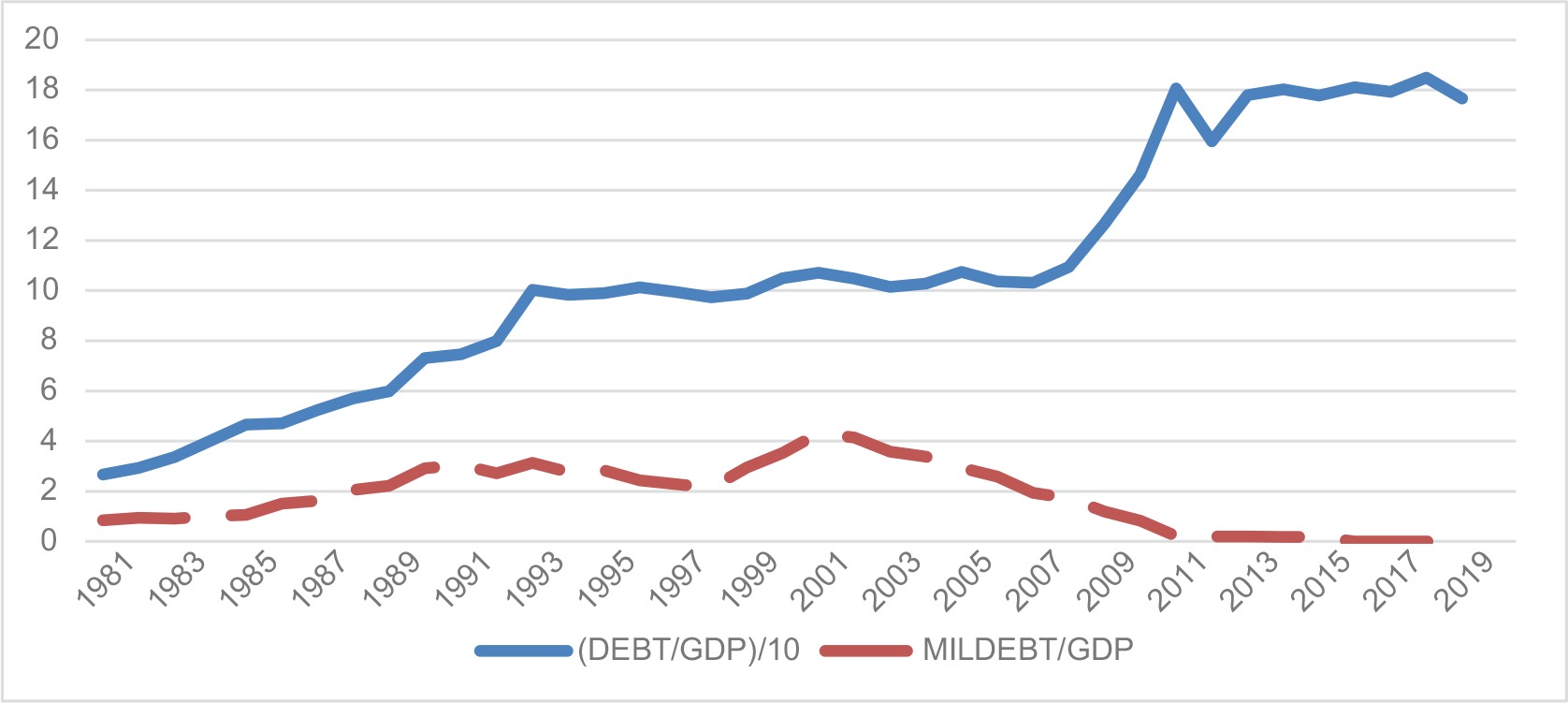
As a result of the above, both the public and the military debt shown in Figure 1, both as a percent of GDP, moved in the same direction until about 1990 when they started diverging, while since the beginning of the 2000s, their relationship changed to being strongly negative. In fact, for the period between 2010 and 2019 when no new orders of major equipment were placed due to the Greek economic crisis, the correlation coefficient between the two variables was strongly negative (-0.85), with the military debt collapsing and the public debt rising dramatically until 2011, after which it stabilised following a smooth positive rate of growth.

Figure 1

Greek total and military debt as percent of GDP. (The public debt figures have been divided by 10 to fit the scale of the diagram).

The analysis that follows investigates the determinants of both the public and military debt and how the two variables are interrelated. For this purpose, we proceed with a brief review of the literature in section 3 and an analysis of the methodology in section 4. The empirical results and their interpretation are discussed in section 5, while our conclusions are presented in the last section of the paper.

Literature Review

The research interest on the relationship between defence spending, economic growth and public debt goes back to the 80s. Michael Brzoska (1983) examined what portion of the Third World countries national debt was attributed to defence equipment imports. The results indicate that the cost of new defence equipment purchases from abroad is half as high as the interest in amortisation of old debt. The fast-rising credit burden of arms imports added a very important dimension for the burden measurement of Third World arms imports. Looney and Frederiksen (1986) distinguished between developing countries that are financially resource constrained, and those that are not, and concluded that there is a direct relationship between defence spending and growth only for those that are not constrained.

In recent contributions, we have not been able to trace papers that link the defence debt, or for that purpose, the armed forces debt to the public debt, either in theory or in individual country studies except Alami (2002). Narayan and Smyth (2007) therefore assessed the effect of defence spending and income on external debt for a group of six Middle Eastern countries. Using Pedroni’s (2004) test for panel cointegration, they found a long-term relationship between external debt, military expenditure, and income. The long-term elasticities derived suggest that a rise in defence spending contributes to an increase in external debt. Dunne et al. (2004) examined to what extent military spending contributed to the external debt of Brazil, Argentina, and Chile during the 1980s. They found no evidence that military burden had any impact on the evolution of debt in Argentina and Brazil, but some evidence that military burden tended to increase debt in Chile. Georgantopoulos and Tsamis (2011), using a cointegration test, investigated the causality between defence spending and external debt for four emerging Northern Africa countries (Morocco, Algeria, Tunisia and Egypt) during the period 1988-2009. The Granger Causality test results using Vector Auto Regression (VAR) estimates and the Error Correction Model implied that there is no dynamic causal link between military expenditure and external debt for all except Egypt, in the case of which they found that a strong unidirectional causality exists running from defence expenditure to external debt. In his very interesting paper, Alexander (2013) found that the defence burden is a statistically significant and economically important determinant of public debt. For this purpose, the author used the Arellano–Bond dynamic panel model for OECD and NATO members over the periods 1988–2009 and 1999–2009. Focusing on the EU countries group, Paleologou (2013) examined the impact of military spending on general government debt using panel data analysis and providing estimates from a dynamic Generalized Method of Moments (GMM) panel model. The results suggested that military expenditure does have a large positive impact on the share of general government debt in the EU. In addition, Esener and Ipek (2015) investigated the effects of defence spending on foreign debt using additional variables such as GDP growth, fixed capital formation and openness. By employing the methodologies of the “Pooled OLS Model” and “Dynamic Panel Estimations” and using annual panel data for 36 developing countries for the period 1996-2013, they found that a change in military expenditure affects external debt positively in the developing countries concerned. Likewise, Azam and Feng (2017), using a sample of ten Asian countries for the period 1990 to 2011, examined the impact of military spending on foreign debt and found that this impact is positive. Focusing on the issue of the debt-management system of 35 arms importing countries, Khan et al. (2021) test the effects of military expenditure on external debt by using annual panel data for the period 1995 to 2016. Their results suggest that defence expenditures increase the external debt burden in the countries included in the study. Specifically, they found that military expenditure tends to increase foreign debt in countries where the debt management system is weak. The authors suggest that such countries need to devise economic policies that restrict their military expenditure, reduce their external debt and improve their economic condition. On the specific NATO group, Karagianni and Pempetzoglou (2019) again employed the linear and non-linear Granger causality methods in order to determine the causal relationship between military expenditures and external debt for the period 1960-2015. Their estimates indicated the existence of linearity in the cases of Greece, Italy, UK and USA and the existence of nonlinearity in the cases of Turkey and the USA.

Turning to papers that examine individual country cases, Karagol (2006) investigated the causal relationship between defence expenditures and external debt for Turkey for the period 1955–2000 by applying a multivariate model. The paper employed a vector error correction model to test for Granger causality in the presence of cointegration between variables and concluded that there is both a long term and short-term unidirectional causality running from defence expenditures to external debt. On the Turkish case again, Sezgin (2004) examined the relationships between Turkey’s defence expenditure and external debt for the period 1979–2000 using Engle–Granger methodology. However, the findings show no clear evidence of defence spending–debt relationships for the period analysed. Shahbaz et al. (2013), investigated the effect of military spending in Pakistan on external debt for the period 1973–2009 using the autoregressive distributed lag bounds testing approach to examine cointegration among the variables. Their findings indicated the existence of cointegration that confirms the presence of a long-term relationship among military spending, external debt, economic growth, and investment. In addition, the results reveal that a rise in military spending increases the stock of external debt. Yemane Wolde-Rufael (2009) finds similar results for Ethiopia,

In the case of Greece, the view that spending on national defence has been one of the leading causes of the Greek debt crisis has been popular in the literature during the past decade. Such concerns have risen following extensive incidents of corruption, especially related to defence procurement cases at the turn of the century. It seems, however, that such issues have been effectively treated via public procurement reforms (Giotopoulos et al., 2015). Given this background, Paparas et al. (2016) attempt to assess the relationship between national defence spending and economic growth. Dimitraki and Kartsaklas (2018) conclude that the primary causes of debt growth in Greece are high deficits, inflation and military spending, a view opposed by Skaperdas (2015). Finally, Nikolaidou (2016) examined the impact of defence spending on the evolution of the Greek debt during the period 1970-2011. Using the ARDL approach to cointegration, she concluded that defence spending and military equipment imports have had an increasing effect on Greek public debt in the short run, while investment has helped to reduce debt both in the short and long term. As a counterargument to these, Alogoskoufis (2021) shows that the Greek public debt has been the result of excessive public and private consumption, following the country’s membership of the EU and, later, of what he calls “Euro Euphoria”.

Methodology

The specification adopts a system of two equations. The first, focusing on the public debt, follows, in broad terms, the one proposed by Alexander (2013), (emphasising the lag structure), Karagol (2006), (specifically on the investment-debt relationship) and Sezgin (2004), (on the defence – debt link). The second equation considers military debt as the dependent variable, using as determinants those of the demand for defence expenditure as proposed by Smith (1980, 1989). This formulation has an advantage over a reduced form equation since it regards the behaviour of military debt separately as this is affected by its own determinants. In addition, once this variable is rendered endogenous, one can consider certain elements of the two-way nature of its complex relationship with DEBT, such as the functional form of the DEBT MILDEBT relationship. The simpler form that can be adopted is the linear one but inspection of the scatter plot (figure 2) of the logarithm of DEBT with the logarithm of squared MILDEBT validates the argument that the relationship could be nonlinear, since the plot assimilates a parabola.

Figure 2

Scatter plot of the relationship of total and military debt as percent of GDP.

The model, therefore, can be expressed as follows with equation (1) taking alternatively a linear and a non-linear form²:

ln(DEBT) = f (GROWTH, BUDGET, ln(GGK), ln(MILDEBT), ln((MILDEBT)²) (1)

ln(MILDEBT) = g (ln(EQDEF), ln(GTR), ln(SP)) (2)

Following Bragoudakis and Zombanakis (2017) and Katsaitis et al. (2019), we use defence spending on equipment rather than the total defence expenditure of the country for two reasons. First, we avoid double counting to a very large extent, in cases in which variables representing the total national budget are included in the model.³ Second, focusing on the defence equipment, we emphasise the technical progress embodied in it and the ensuing stimulating effects on private investment in R&D (Herrera and Gentilucci, 2013; Kennedy, 1987). Since Greece imports most of its defence equipment, the use of this specific variable underlines the failure to take advantage of significant technological transfers.

The empirical method adopted to estimate the described system of simultaneous equations is 3SLS, an approach developed by Zellner and Theil (1962) that controls endogeneity and simultaneity. The method assumes the existence of cross-equation correlation through correlation of their error terms. Clearly, the determination of the public and military debt in Greece depends on a number of interrelated factors which are embodied in the error terms, such as geopolitical variables. If the specification incorporates this information, it produces more efficient estimates. The sample covers a long period starting at 1980 until 2021 and data is annual. The sources and the definition of the variables used to estimate (1) and (2) are given in Table 1.

Empirical Results and interpretation

Descriptive statistics of all the variables in the analysis are included in Table 2 below. GROWTH and BUDGET present the largest variability but the probability that they follow a normal distribution is high. Further, the probability of accepting the null hypothesis that ln(MILDEBT) and ln(GGK) are normally distributed is the lowest among the variables included.

To consider the dynamic nature of the variables like public debt and economic growth and avoid problems such as spurious correlation, we use the Augmented Dickey Fuller (A.D.F.) test Dickey and Fuller, 1979) on all the variables considered for the existence of a unit root. The test rejects the unit root hypothesis for all variables except the MILDEBT and SP. For these, the hypothesis of a unit root is rejected using the unit root test that assumes the existence of a structural break (the existence of which is confirmed by inspection of their graphs).⁴ As a result, since all the variables are stationary, we use them in levels in the estimations and to take care of any heteroscedasticity problems, we express them in logarithms.

Table 3 shows the 3SLS estimates of the system of the two equations (1) and (2). In the first column the first equation of the system is estimated assuming a linear relationship between DEBT and MILDEBT, while the second column includes estimates of the first equation considering the existence of a quadratic relationship between the two variables. As instruments, we use the demeaned variables squared lagged once and the product of the variables taken two at a time (see Bound et.al., 1995).

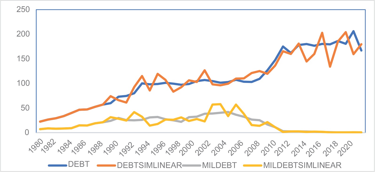
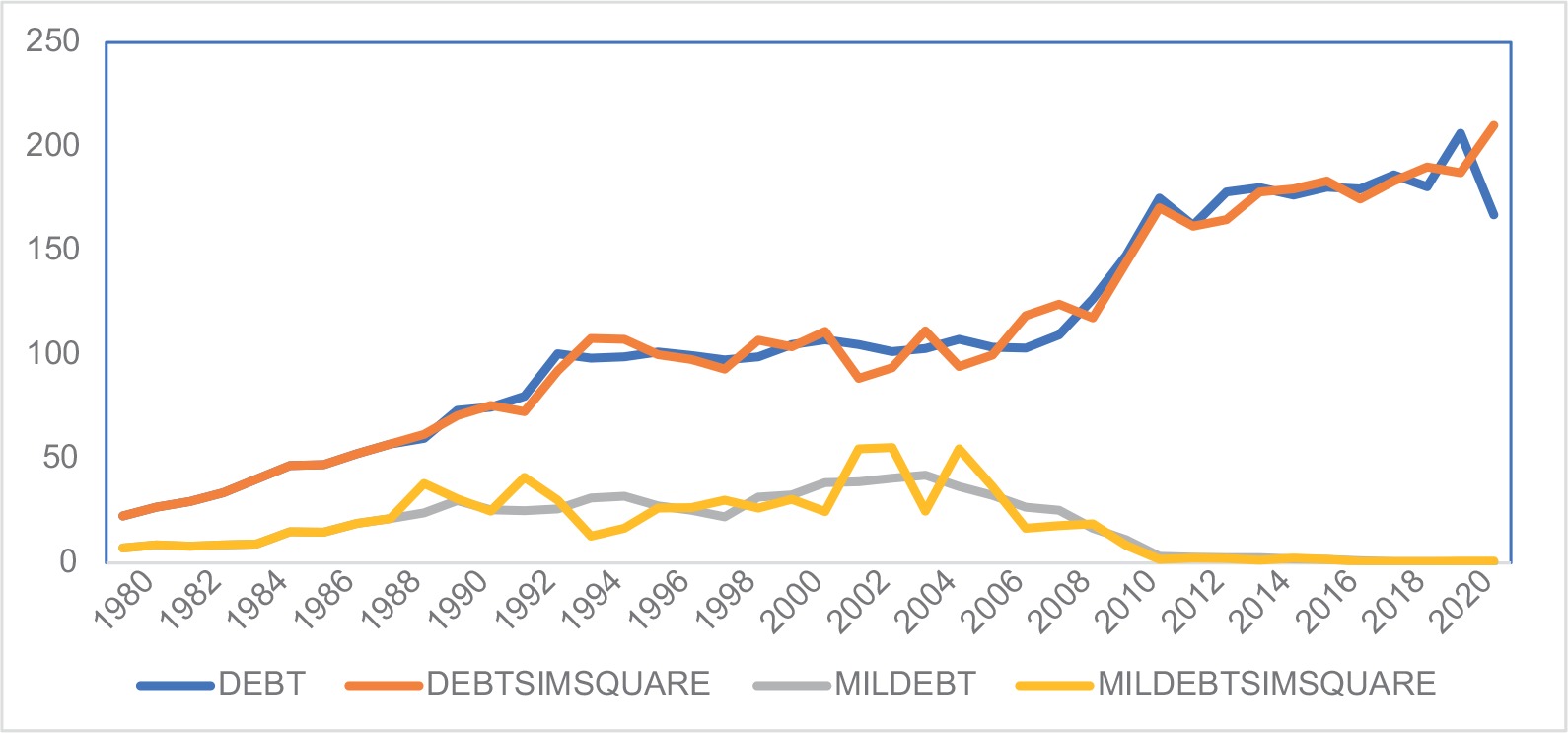
The table also reports the corresponding diagnostic tests (Potrmanteau test⁵ for autocorrelation and Jarque-Bera test for normality of the residuals). The null of no autocorrelation is rejected and some non-normality is detected in the linear version. The diagnostics of the non-linear model show no autocorrelation and no non-normality, which renders this version preferable to the one adopting the linear specification. In addition, the quadratic version yields higher adjusted R² coefficients. The diagrams of the simulations of the two estimated models are shown in Figures 3 and 4. The better forecasting performance of the non-linear fitted model as compared to the linear can be assessed using these graphs.

Figure 3

Actual and simulated public and military debt assuming a linear relationship.

Figure 4

Actual and simulated public and military debt assuming a quadratic relationship.

In both versions, all coefficients are significant, bearing the expected signs. In both models, focusing on the second equation, a substantial part of defence spending on equipment (between 50% and 80%, given the log version of the model) burdens the military debt as expected. The considerable time lag required to do so accounts for the time-consuming procedures required and the political cycle sometimes involved in such cases. However, when moving to the first equation, as a follow up to the developments regarding the military debt, one can see that its impact on the public debt of the country is strongly inelastic. The findings of the non-linear model corroborate the resulting inelastic behaviour of the public debt of Greece to changes to the military debt. In fact, the estimated quadratic relationship of DEBT and MILDEBT forms a parabola (since the coefficient of the squared term is negative). This entails that increases in MILDEBT cause a respective increase in DEBT, although at a declining rate, thus making it negligible in the long run.

Turning to economic growth and investment increases, these lead to a reduction in the public debt over the sample period in both versions, revealing, however, low responsiveness. Similarly, the response of the public debt to changes in the budget is significant, but rather weak, a finding related to the alleged statement that the fiscal consolidation and the structural reforms that took place during the debt crisis did not have the desirable effect on the debt to GDP ratio.⁶ The military debt, on the other hand, is affected positively by the Greek government’s spending on equipment, as pointed out earlier, the threat represented by Turkish defence spending and the spill-over effects due to the country’s NATO membership. The impact of these variables on the military debt takes a long time to materialise, mostly due to the complicated recording procedures involved, as described in section 2 above, as well as to the arms race between Greece and Turkey (Andreou and Zombanakis, 2006).

Conclusion

This paper has focused on assessing the impact of defence equipment procurement expenditure on the public debt of Greece. Given that the relevant recording procedure has undergone a variety of serious modifications over the years, the assessment of the burden on the public debt of Greece cannot be based on a straightforward accounting basis. We have thus used a two-equation model to emphasise the defence debt specification rather than treating it as a simple determinant in a public debt equation This approach has aimed at considering simultaneity, thus contributing to the efficiency of the estimators.

Our findings using both the linear and the non-linear relationship indicate that the response of the public debt to changes in the defence debt may be positive, although much weaker than what has been considered in the literature so far, with Brzoska (1983) and Alami (2002) being the only papers that consider the direct link between military and public debt. The remaining papers in the literature tend to argue that there is a positive relationship between defence expenditure and public debt, either in theoretical terms or dealing with individual country cases, except Skaperdas (2016) and Shahbaz et al. (2013). Moreover, given that the empirical results are in favour of a non-linear, quadratic, response of the public debt to increases in the military debt, it is argued that the resulting burden which is caused diminishes overtime and tends to become negligible in the long run thanks to the prolonged payments schedules.

The underlying facts explain and support our conclusion: The last order placement for the procurement of major equipment by the Hellenic Armed Forces occurred in 2004. Since then, with the economic crisis period starting in 2009, there was no room left for further defence equipment purchases for the entire period under consideration.

Last, but not least, a useful comment on definitional matters: Military weapon systems are considered as fixed assets, with their acquisition recorded as gross fixed capital formation, i.e., as capital expenditure. Given that the Greek debt crisis has been mainly the result of excessive consumption, as pointed out earlier, one can hardly consider that aiming at national security via investing in defence equipment would be regarded as a cause for excessive consumption and, consequently, a burden on the country’s public debt.