
Introduction
The widespread geopolitical tensions caused by Russia’s invasion of Ukraine have recently reignited research interest in the economic ramifications of military alliances in general, and the North Atlantic Treaty Organisation (NATO) in particular. Theoretical and empirical debates focus on the factors affecting the contributions of military alliance members to the defence expenditure of the alliance, splitting researchers into advocates of free-riding arguments and supporters of the complementarity of defence spending decisions among alliance members.
In this context, the present study re-examines the theory of alliances to incorporate spillovers associated with each alliance member by introducing the idea of net spills measured as the difference between spill-ins and spill-outs, with specific reference to NATO’s remarkably durable and sizeable military alliance. We study seven NATO members, namely the United States, the United Kingdom, the Netherlands, Germany, Italy, Greece, and Türkiye, over the 1971–2022 period to depict the net spills contribution of each member to the alliance with the use of time-varying dynamic quantile connectedness analysis. We contribute to the growing literature on the economics of military alliances, as, to the best of our knowledge, this is a novel methodological approach, both theoretically and empirically, deployed for assessing the impact of the spending decisions of military alliance members.
The conclusions that stem from testing our theoretical model reveal strong incentives among the allies for free-riding behaviour due to the costly spill-outs added to the cost of defence equipment acquisition. Our findings also suggest that the North-European NATO member states included in our sample tend to be net contributors to the alliance, while the South-European member states tend to be net receivers. It also seems that NATO member states are only motivated to contribute during crisis periods, a finding that has gained more significance in light of the war in Ukraine.
The rest of the paper is organised as follows. Section 2 presents a brief overview of recent pertinent studies. Section 3 deals with the development of our theoretical model and Section 4 contains the statistical properties of our data and econometric methodology. Section 5 presents the empirical findings. Finally, Section 6 sums up our findings and draws conclusions from them.
Prior Research
Following Olson and Zeckhauser (1966), who put forward military alliances as collectively owned and collectively consumed public goods, the economics of military alliances have been well researched along two main lines of thinking.
The first line comprises researchers who focus on the free-riding challenges that inevitably develop in military alliances due to their public good nature, with smaller members reducing defence spending and big members ending up being consistently net donors to the alliance, as in NATO (Lanoszka, 2015; George and Sandler, 2018; Kim and Sandler, 2020; Palmer, 1990; Sandler and Forbes, 1980). Since its inception, this “exploitation hypothesis” has been applied to a variety of international collective action scenarios, including regional integration schemes (see, for example, Sandler and Hartley, 2001). The theoretical extensions of the “weakest link” and the “best shot” models are discussed in Sandler (1993). The “weakest link” explanation places emphasis on the smallest provision level of the alliance determining the defence level of the entire alliance, as alliance members tend to match the defence contributions of the smallest contributor. In contrast, the “best shot” proposition suggests that the security level of the entire alliance depends upon the largest member’s spending, thus rendering spending on the part of smaller members redundant. A number of studies deploy spatial analysis to unravel the importance of physical proximity, as well as trade connectivity, among military allies (Flores, 2011; Skogstad, 2016; Yesilyurt and Elhorst, 2017). Among these, a recent study on NATO by George and Sandler (2022) uncovers allies free-riding on the aggregate military expenditure of other allies. The authors attribute free-riding to reliance on the defence spending of NATO allies that are physically close to Russia, although they do stress that this pattern appears to have been reversed, with the enhanced Russian threat that NATO allies now perceive, limiting the incidence of free-riding to a certain extent.
A second line of explanation focuses on the fact that the sheer nature of defence systems and their use by alliance members encourage substantial cooperation by allies. According to this approach, military alliances have tended to be characterized by increasing complementarity in member defence spending decisions since the early 1970s (see, for example, Beron et al. 2003; Gonzalez and Mehay, 1991; Sandler and Forbes, 1980; Sandler and Murdoch, 1986). Although free-riding does not completely disappear, alliances are characterized by greater complementarity, with members sharing defence costs, rather than the cost falling for the most part on larger members of the alliance. Gates and Terasawa (2003) develop a model that treats alliance defence expenditures as private goods, introducing publicness through commonality of interest and commitment among allies. They find that the net benefits of alliance membership depend on the commonality of interest among alliance members, their commitment to one another and the adversaries’ perceptions of the threat posed by the alliance. Plümper and Neumayer (2015) suggest that the incidence of free-riding in military alliances must take into account the responsiveness of smaller allies to growth in the military spending of two superpowers. Thus, incentives to free-ride do not simply result from the total defence spending of a big member of the alliance, the United States, but also, and perhaps more importantly, from changes in the defence spending of the United States and the then Soviet Union over time. In the case of NATO, free-riding is attributable to members’ feeling of security, rather than size, with countries responding both to the growth in American military spending on the one hand, and the growth of Soviet spending on the other between 1956 and 1988. More recently, Alley (2021), who studies 204 alliances from 1919 to 2007, finds little evidence to support the free-riding hypothesis, attributing low defence spending to allied capability or efficiency gains from specialising in pooled military resources.
The Theoretical Framework
In this section, we expand the economic theory of alliances (Olson and Zeckhauser, 1966), modifying a model that borrows from George and Sandler (2018, 2021, 2022), to incorporate the spills that stem from the obligations of each ally by introducing the notion of spill-outs of ally i, derived from its defence expenditure and diffused into the N-1 allies and the notion of net spills, namely the difference between spill-outs and spill-ins.
The Theory of Alliances
The economic theory of alliances developed by Olson and Zeckhauser (1966) touches upon a number of issues, notably those related to burden sharing and interaction between members. In its original form, the concept of an alliance is taken to represent security and, along with it, defence spending as a pure public good.1 In this context, several public finance issues arise, such as non-rivalry and non-excludability, which, in their turn, lead to considering problems like unequal burden sharing and, consequently, free-riding possibilities, to which the literature refers as the “exploitation hypothesis” (Olson and Zeckhauser 1966; Sandler and Hartley 1995, p. 23). Once this is the alliance environment, one can then argue that defence expenditure for each ally, as well as in the overall context, is sub-optimal in terms of Pareto optimisation, pointing instead to the direction of a Nash equilibrium.2
In technical terms, following George and Sandler (2018, 2021, 2022), the welfare function of each ally can be expressed as depending on the consumption of a non-defence good ci, the collective defence good
and the external threat T. Therefore, the welfare function takes the following form:
Sandler (1977) extended the analysis by proposing a joint product model, for which the defence expenditure of an ally can produce either public output or private output. Sandler and Hartley (1995, pp. 35–36) distinguish between the demand functions of a pure public good and the joint product model by using the concept of what they call “full income,” which incorporates the sum of both income and spill-ins enjoyed by an alliance member. Thus, in the case of a joint product model, the income constraint, including the spill-in benefits p
where Qi is the total defence output of the alliance.
Expanding the Economic Theory of Alliances: A Net Spills Approach
A basic assumption of the standard economic theory of alliance (Sandler and Hartley, 1995, p.22) is that ally i receives spill-ins, derived from the defence expenditures of its N-1 allies, as follows:
Where qk represents the defence expenditures of the N-1 allies, but
However, in the context of an alliance, ally i has to meet certain obligations, which imply that some of the defence part of each member’s defence expenditure is devoted to infrastructure and other operating expenditures to support the alliance’s needs. To incorporate the spills that stem from the obligations of each ally, we expand the standard economic theory of alliance by focusing on the concept of the spill-outs of ally i, representing some of its defence expenditure and directed to the remaining N-1 allies, as follows:
where qt represents the defence expenditure of ally i, and
Substituting Equations (1) and (2) into Equation (3), we get the net spills constraint:
We interpret the net spills as the difference between the spills provided by ally i to other allies and the spills received by ally i from other allies. In other words, the net spills show the net contribution of each member to the common security good produced by the alliance. A positive value of net spills from ally i to other members of the alliance implies that the ally is a net provider of security spills and the allies are net receivers in their relationship with ally i, while the opposite holds for negative values of net spills.
We assume a political realism approach, according to which each country gains utility from spill-ins and loses utility from spill-outs. The political realism assumption argues that the international system consists of states that aim to overpower other rival states and thus dominate in the international power hierarchy (Hobbes, 1946, p.82; Morgenthau, 1985, p.12). In that sense, power is a tool for a state to serve its national interest and overcome the consequences of security dilemma (Hertz, 1951), as this is rooted in the anarchy of the state system (Sørensen et al., 2022, pp. 67–102). In a political realism environment, it is straightforward to assume that even in a military alliance, each state seeks to serve its own interest, thus determining its behaviour in the alliance by considering not only the possible spill-ins but the spill-outs too, as expressed by Equation (4). Extreme negative values of net spills may be interpreted as possible free-riding, given that the ally concerned receives more security spills than it provides to the alliance.
The social welfare of ally i is given by the following function:
In Equation (5), let
Substituting the net spills constraint of Equation (1) and the budget constraint into Equation (5), we get ally’s i maximization problem, with respect to its defence spending as follows:
The first-order conditions of the above equation give:
z denotes the fraction of the military spending of ally i that has not been devoted to support the alliance’s needs.
Rearranging the above First-Order Conditions (FOC) gives:
The interpretation of Equation (8) suggests that the lower the z and/or the higher the p, the more expensive Qi, the amount of defence good consumed by ally i. However, z represents ally’s i remaining fraction of defence spending after spill-outs have been subtracted. Therefore, according to Equation (8), a lower value for z (indicating a higher value of spill-outs) increases the cost of defence. Consequently spill-outs increase the defence costs for ally i, thus playing the same role as the price p of the defence.
Further, applying the total differential in Equation (7), we get:
which indicates free-riding, namely when the other allies, except for ally i, increase spending, then ally i decreases its defence spending. Therefore, the larger the spill-ins from the other allies to ally i, the higher the incentive for free-riding, as in George and Sandler (2021). Consequently, introducing the notion of spill-outs in our model confirms the free-riding incentive.
Data Statistical Properties and Econometric Methodology
Description of Variables
In the analysis, we employ yearly data concerning military spending on equipment as a percentage of the total military expenditure for seven NATO members (the United States, the United Kingdom, the Netherlands, Germany, Italy, Greece, and Türkiye) over the period of 1971–2022. The data was obtained from NATO’s database,3 and the above countries were selected on the basis of the availability of data due to their long-standing membership of the alliance. Table 1 provides summary statistics for the variables. The statistical properties of the series indicate a non-normal distribution, since the kurtosis is lower than 3 in all cases (platykurtic distribution), except for the United States and Türkiye, where we can see a kurtosis close to 3. The values for skewness also provide evidence in favour of a non-normal distribution, as in most cases it is either higher than 0.5 or lower than –0.5. In addition, the Jarque–Bera (JB) normality test rejects the null hypothesis of normal distribution of the time-series, except for the cases of Greece and Türkiye. When it comes to unit-root, we can see that according to the augmented Dickey–Fuller (ADF) test, we cannot reject the null hypothesis of a unit-root, with the exception of Türkiye, implying that the variables are non-stationary in levels, which is a strong sign of mean aversion behavior that justifies the use of non-linear econometric techniques.
Table 1
Summary statistics for the variables and Jarque–Bera normality test and ADF test.
Notes: *, **, and *** denote significance at 10%, 5%, and 1% level, respectively.
Furthermore, the quantile-mean covariance (QC) normality test (Bera et al., 2016) results, as shown in Table 2, rejects the null hypothesis of normality overall, thus indicating the asymmetric behavior of all series distribution.
Table 2
Quantile-mean covariance (QC) normality test.
Notes: *, **, and *** denote significance at 10%, 5%, and 1% level, respectively. T1, T2, and T3 refer to Bera et al. (2016) statistics:
where
Econometric Methodology
The analysis of the defence spending data revealed the existence of possible asymmetric features, as in Palaios and Papapetrou (2023). The latter indicates the need for applying econometric techniques that allow us a more comprehensive description of the conditional distribution than the ordinary mean approach, thus offering a more robust econometric technique methodology in the presence of conditional heterogeneity and departures from the Gaussian conditions. Therefore, to test the empirical implications and the validity of our theoretical model, we estimate the spillover effects among the selected NATO allies by initially applying the static and dynamic connectedness -analysis developed by Diebold and Yilmaz (2009, 2012, 2014), and thereafter the quantile connectedness methodology developed by Ando et al. (2022), which allows an in-depth analysis of spill-ins, spill-outs and net spills across the whole distribution of our time series.
Static and dynamic connectedness analysis
To estimate the degree of connectedness among NATO allies, we initially apply the methodology developed by Diebold and Yilmaz (2009, 2012, 2014) by considering a covariance stationary N-process Var(p),
where
where
To derive the associated h-step ahead of forecast error variance decomposition, we employ a rolling window, which allows us to examine the dynamics of the spills over time.
Quantile connectedness analysis
At a second step, we apply the quantile connectedness approach developed by Ando et al. (2022), to estimate the spills among NATO allies at various quantiles of the distribution (Antonakakis et al., 2019; Bouri et al., 2021; Chatziantoniou and Gabauer, 2021; Palaios and Papapetrou, 2022). The corresponding measures of the network topology at the τ-th quantile are given by:
where
where
where
Empirical Results and Discussion
Total spillover effects and cohesion in the NATO alliance
In this section, we examine the evolution of the spills produced by the common defence good of the alliance. As a measurement for that purpose, we use the TSI evaluated at various quantiles. We interpret the TSI as the total spills available, stemming from the military expenditure of the alliance’s members that consist the common good of defence. An increase (decrease) in the level of the TCI is an evidence that the available security spills increase (decrease). Consequently, the index indicates the overall ability of the alliance to provide its members with a higher level of security during periods of crisis. In this context, it is straightforward to interpret an increase (decrease) in the TSI as an increase (decrease) in the cohesion and effectiveness of the alliance, as more (less) spills are the result of a higher (lower) level of security provision from the alliance to its members.
Figure 1 illustrates the variation of the TSI index evaluated at the mean and various quantiles along the conditional distribution. The quantile approach captures the impact of negative and positive political and geopolitical shocks in the international system of a different magnitude. As the spills primarily stem from the military expenditure of the allies, we interpret negative shocks (lower quantiles) as beneficial shocks (peace event) related to a lower level of military expenditure, and positive shocks (upper quantiles) as adverse shocks (crisis event) related to a higher level of military expenditure. Therefore, a period of geopolitical crisis is associated with a positive (adverse) shock that corresponds to the right-tail dependence of the conditional distribution, while the opposite holds for a peaceful event that is associated with a negative (beneficial) shock that corresponds to the left-tail dependence of the conditional distribution. The empirical evidence, presented in Figure 1, reveals an overall increasing trend of the TSI as we move from the lower to the upper quantiles. Specifically, in the case of a peaceful event, quantiles (τ = [0.10, 0.20, 0,30]), the values of the TSI are (62.2, 64.3, 69.0), while in the case of a normal geopolitical period, quantiles (τ = [0.40, 0.50, 0.60]), the values of the TSI are (73.4, 75.1, 75.4). Finally, in the upper tail of the distribution, which corresponds to a crisis event taking place, (τ = [0.70, 0.80, 0.90]), the values of the TSI are (76.2, 79.3, 81.8). The findings above align with the behavior of an effectively working alliance during crisis periods. The spills produced by the alliance for consumption by their members increase during these times. We interpret this as evidence that some selected members are motivated to contribute only during periods of crisis. This conclusion has been further reaffirmed since the onset of the war in Ukraine.
Figure 1
Total Spills Index (TSI) evaluated at the mean and various quantiles along the conditional distribution. The horizontal line is the TSI estimated at the conditional mean.
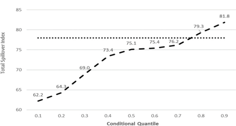
Further, we observe that the growth rate of the TSI, which is interpreted as the responsiveness of the alliance to exogenous geopolitical shocks, decreases at a higher rate after a beneficial shock (peaceful event), compared to the rate at which it increases after an adverse shock (crisis event). The above finding implies that despite the increasing trend of the TSI, as we move from the lower to the upper quantiles, there is space for improvement when it comes to the cohesion of the alliance during normal and peaceful periods.
Total spillover effects and cohesion among NATO allies
In this section, we apply the connectedness methodology to empirically examine our model, detecting net spillover effects among NATO members included in our sample. We examine the net directional connectedness between the allies of our model. We interpret the net directional connectedness as the difference between the spills provided by ally i to others allies and the spills received by ally i from the other allies
Table 3 shows the various connectedness measures estimated at the median (τ = 0.5). We observe that as expected, the United States is the largest security spills contributor of our system
Table 3
System connectedness evaluated at the median (τ = 0.5).
Notes: The ij-entry of the upper left 6×6 variable sub-matrix gives the ij-th pair-wise directional connectedness. The right-most (FROM) column gives total directional connectedness from all other variables to i variable. The bottom (TO) row gives total directional connectedness to all other variables from j variable. The bottom-most (NET) row gives the difference in total directional connectedness (to - from). The bottom right element, in bold, is total connectedness.
Overall, during normal periods, the United States and the northern allies (the United Kingdom, the Netherlands, and Germany) are net providers of security spills, while the southeastern allies (Italy, Greece, and Türkiye) are net spills receivers. Therefore, our empirical results, in line with George and Sandler (2018, 2022) and the predictions of our theoretical model stated in Equation (5), support the possible free-riding behavior of some NATO allies, as they receive more spills than the spills they provide. It should be noted that a small negative value of net spills does not necessarily imply free-riding behavior, as it could be attributed to a disproportionately high level of spills provided by the dominant ally (United States). In contrast, an extreme negative value of net spills reinforces the indication of free-riding behavior. The empirically verified free-riding behavior during the normal period is alarming as it indicates insufficient military preparation, thus explaining the failure to deter Russia from invading Ukraine, in line with the findings of George and Sandler (2022).
To examine the dynamics of the system, we plot the time-varying evolution of the TSI evaluated at the conditional median (τ = 0.50) and the right-tail dependence (τ = 0.90) of the conditional distribution, which corresponds to positive shocks, namely to adverse political or geopolitical events that increase the tension between NATO and its adversaries (Figure 2). We see that the total spill effects (TSI) are of greater magnitude for adverse political or geopolitical shocks (τ = 0.90) (right-hand graph) than for normal periods. Specifically, our empirical results in the right-tail dependence (Figure 2B) are consistent with a higher magnitude of security spills after the Gulf War (1990–1991), the September 11th, 2001 attacks in the United States, the War in Afghanistan (2001), and the Iraq War (2003). Further, we can see a gradual decrease of spills between 2010 and 2015, which can be explained by the gradual de-escalation of the war in Iraq and a decrease after 2015 because of the disengagement of the United States from the war in Afghanistan. The evolution of the TSI evaluated at the average connectedness exhibits similar patterns that are accompanied, however, by spills, as expected, of lower intensity. It should be noted that the increase in the spills that happened during the period of the Russian invasion of Ukraine is pronounced in the media quantile (τ = 0.5, left-hand side graph), rather than the right-tail dependence (τ = 0.9, right-hand graph), as expected. This finding is related to the fact that the reaction of the alliance to the Russian invasion of Ukraine is characterised by a low profile and an indirect engagement in order to avoid an escalation of conflict between NATO allies and Russia.
Figure 2
Measures of dynamic total spills at median (τ = 0.50) and right-tail (τ = 0.90) of the conditional distribution (A) Dynamic total spills at the tenth conditional quantile (τ = 0.50). (B) Dynamic total spills at the ninetieth conditional quantile (τ = 0.90)
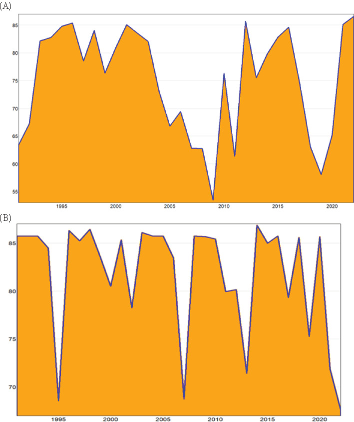
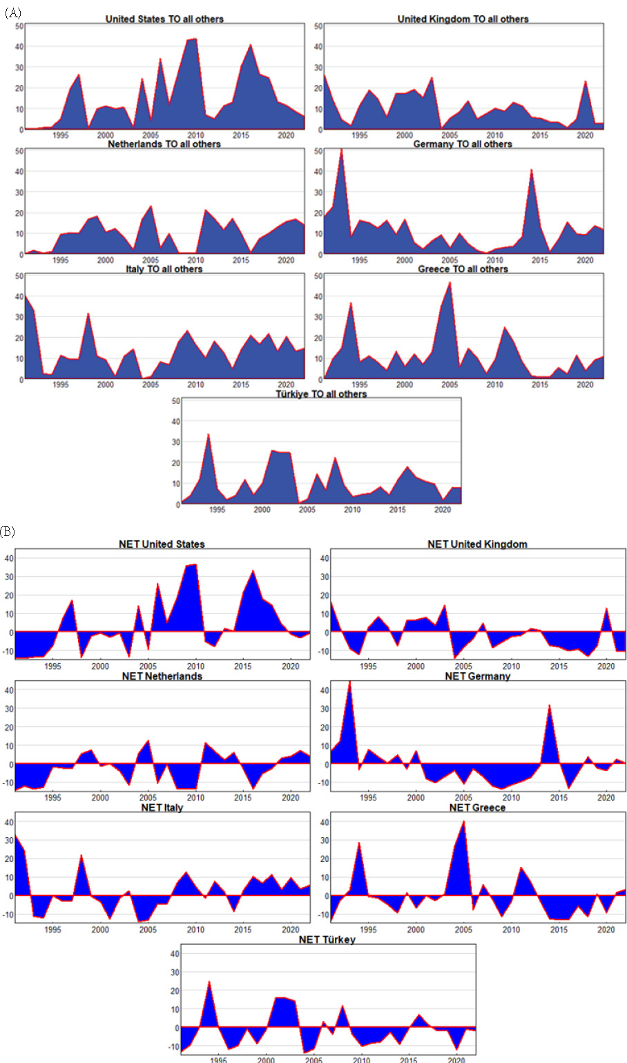
Figure 3 shows the evolution of dynamic spills evaluated at the right-tail dependence of the conditional distribution. Specifically, when it comes to the dynamic total directional spills from ally i to others (Figure 3A), we see that for the entire period depicted, the United States is the major spills provider to the rest of the allies at an increasing magnitude after the terrorist attacks of 9/11 up to 2016, when we observe that there was a relative shift in the United States’ stance concerning NATO. As a result, spills from the United States to other allies decreased thereafter. Our findings regarding the United States are also consistent with the general low-profile engagement of NATO allies in Russia’s invasion of Ukraine, as a low degree of spills from the United States during that period is evident. The same conclusions could be extracted by the evolution of the dynamic net total directional spills of the United States (Figure 3B). We also see a gradual decrease in both total directional spills from the United Kingdom to other allies and net total directional spills of the United Kingdom after the mid-2000s, which becomes more intense after Brexit, except for the period 2019–2021, which can be interpreted as spills stemming from the defence policy of the newly elected government, mostly because of the pressure on the United Kingdom to increase its defence spending to meet its NATO obligations. For the Netherlands, Germany, and Italy, we see mixed results, where periods of positive alternate with periods of negative net spills. For Greece, our results are consistent with a negative net spills effect after the 2008 economic crisis, which seems to change to a positive spills effect after 2020, because of the gradual restoration of macroeconomic and fiscal stability. Finally, we observe that Türkiye’s net spills contribution can be divided into two distinct periods, namely a period before and a period after the beginning of the 2010s, which could be interpreted as a gradual shift in the country’s defence policy.
Figure 3
Dynamic spills evaluated at the right-tail dependence (τ = 0.90) (A) Dynamic total directional spills from ally i to the other allies at the right-tail of the distribution (τ = 0.90). (B) Dynamic net total directional spills for ally i at the right-tail of the distribution (τ = 0.90)
Overall, our theoretical model incorporates not only the spill-ins but also the spill-outs, namely the spill cost that stems from the obligations of each ally. Our empirical results, in line with the predicted free-riding behaviour of our theoretical model, provide evidence in favour of free-riding of the northeastern member states due to the costly spill-outs added to the cost of acquiring defence equipment. Our findings suggest specifically that the North-European NATO member states included in our sample tend to be net contributors to the alliance, while the selected South-European member states tend to be net receivers. It also seems that the selected NATO member states are only motivated to contribute in crisis periods, a finding that may indicate insufficient military preparation and has been more evident in light of the war in Ukraine. The above findings are in line with the predictions of the seminal model of Olson and Zeckhauser (1966) and Plümper and Neumayer (2015) as well as with the more recent evidence provided by George and Sandler (2022). The latter concluded that the pattern of free-riding and lack of response to heightened Russian defence spending probably encouraged the invasion, as NATO appeared divided. On the other hand, our results are in contrast with those of Alley (2021) who finds that free-riding behavior based on economic weight is unusual in alliance politics, which may be due to limits on security as a public good or bargaining between alliance members. Finally, the above empirical analysis consistently interprets the major geopolitical events of the examined period.
Conclusions
This paper is focused on the degree of interaction in a sample of NATO member states under a variety of external circumstances and threat intensity. We contribute to the pertinent literature in the following ways. Firstly, by enriching the theory of alliances, in which we incorporate the net spills between alliance members defined as the difference between spill-out and spill-in effects. Secondly, by testing our model empirically, deploying dynamic connectedness analysis to examine net spills among seven members of the NATO alliance. Specifically, the empirical assessment is tested via the application of the time-varying dynamic quantile connectedness analysis. To the best of our knowledge, quantile connectedness methodology has not been implemented before in the field of defence economics to measure the spills among countries. The conclusions drawn point to the fact that there is a pronounced tendency for free-riding among the selected alliance members due to the costly spill-outs added to the cost of equipment acquisition. Our findings also suggest that the North-European NATO member states included in our sample tend to be net contributors to the alliance, while the South-European member states tend to be net receivers, thus exhibiting free-riding behaviour. Finally, it seems that some NATO member states are motivated to contribute only during period of crisis. This is a conclusion that has been reaffirmed since the war in Ukraine began.